Multiple OLS Estimation
Multiple Regression via lm()
To estimate a multivariate model in R, we can use the
lm()function:- the tilde (
~) separates the dependent variable from the independent variables; - independent variables must be separated by
+; - the constant term (
$\beta_0$) is included automatically by
lm(). To remove it, include0in the formula.
- the tilde (
Example 3.1: Determinants of College GPA in the United States (Wooldridge, 2006)
- Consider the variables:
colGPA(college GPA): average college grade point average;hsGPA(high school GPA): average high-school GPA;ACT(achievement test score): the score on the college entrance achievement test.
- Using the
gpa1dataset from thewooldridgepackage, we estimate the following model:
$$ \text{colGPA} = \beta_0 + \beta_1 \text{hsGPA} + \beta_2 \text{ACT} + u $$
# Load the gpa1 dataset
data(gpa1, package = "wooldridge")

# Estimate the model
GPAres = lm(colGPA ~ hsGPA + ACT, data = gpa1)
GPAres
##
## Call:
## lm(formula = colGPA ~ hsGPA + ACT, data = gpa1)
##
## Coefficients:
## (Intercept)        hsGPA          ACT
##    1.286328     0.453456     0.009426
- We can inspect the estimation in more detail by applying
summary()to the object returned bylm():
summary(GPAres)
##
## Call:
## lm(formula = colGPA ~ hsGPA + ACT, data = gpa1)
##
## Residuals:
##      Min       1Q   Median       3Q      Max
## -0.85442 -0.24666 -0.02614  0.28127  0.85357
##
## Coefficients:
##             Estimate Std. Error t value Pr(>|t|)
## (Intercept) 1.286328   0.340822   3.774 0.000238 ***
## hsGPA       0.453456   0.095813   4.733 5.42e-06 ***
## ACT         0.009426   0.010777   0.875 0.383297
## ---
## Signif. codes:  0 '***' 0.001 '**' 0.01 '*' 0.05 '.' 0.1 ' ' 1
##
## Residual standard error: 0.3403 on 138 degrees of freedom
## Multiple R-squared:  0.1764,	Adjusted R-squared:  0.1645
## F-statistic: 14.78 on 2 and 138 DF,  p-value: 1.526e-06
OLS in Matrix Form
Notation
For more details on matrix-form OLS, see Appendix E of Wooldridge (2006).
Consider the multivariate model with $K$ regressors for observation $i$: $$ y_i = \beta_0 + \beta_1 x_{i1} + \beta_2 x_{i2} + … + \beta_K x_{iK} + u_i, \qquad i=1, 2, …, N \tag{E.1} $$ where $N$ is the number of observations.
Define the parameter column vector, $\boldsymbol{\beta}$, and the row vector of explanatory variables for observation $i$, $\boldsymbol{x}_i$: $$ \underset{1 \times K}{\boldsymbol{x}_i} = \left[ \begin{matrix} 1 & x_{i1} & x_{i2} & \cdots & x_{iK} \end{matrix} \right] \qquad \text{e} \qquad \underset{(K+1) \times 1}{\boldsymbol{\beta}} = \left[ \begin{matrix} \beta_0 \\ \beta_1 \\ \beta_2 \\ \vdots \\ \beta_K \end{matrix} \right],$$
Notice that the inner product $\boldsymbol{x}_i \boldsymbol{\beta}$ is:
- Therefore, equation (3.1) can be rewritten, for $i=1, 2, ..., N$, as
$$ y_i = \underbrace{\beta_0 + \beta_1 x_{i1} + \beta_2 x_{i2} + … + \beta_K x_{iK}}_{\boldsymbol{x}_i \boldsymbol{\beta}} + u_i = \boldsymbol{x}_i \boldsymbol{\beta} + u_i, \tag{E.2} $$
- Let $\boldsymbol{X}$ denote the matrix containing all $N$ observations for the $K+1$ explanatory variables:
- We can then stack the equations for all $i=1, 2, ..., N$ and obtain:
Analytical Estimation in R
Matrix/Vector Operations in R
- First, let us review the matrix and vector operations used in R:
- Transpose of a matrix or vector:
t() - Matrix or vector multiplication (inner product):
%*% - Inverse of a square matrix:
solve()
- Transpose of a matrix or vector:
# As an example, create a 4x2 matrix A
A = matrix(1:8, nrow=4, ncol=2)
A
##      [,1] [,2]
## [1,]    1    5
## [2,]    2    6
## [3,]    3    7
## [4,]    4    8
# Transpose of A (2x4)
t(A)
##      [,1] [,2] [,3] [,4]
## [1,]    1    2    3    4
## [2,]    5    6    7    8
# Matrix product A'A (2x2)
t(A) %*% A
##      [,1] [,2]
## [1,]   30   70
## [2,]   70  174
# Inverse of A'A (2x2)
solve( t(A) %*% A )
##          [,1]     [,2]
## [1,]  0.54375 -0.21875
## [2,] -0.21875  0.09375
Example: Determinants of College GPA in the United States (Wooldridge, 2006)
We want to estimate the model $$ \text{colGPA} = \beta_0 + \beta_1 \text{hsGPA} + \beta_2 \text{ACT} + u $$
Using the
gpa1dataset, we create the dependent-variable vectoryand the matrix of independent variablesX:
# Load the gpa1 dataset
data(gpa1, package = "wooldridge")

# Create vector y
y = as.matrix(gpa1[,"colGPA"]) # convert the data-frame column into a matrix
head(y)
##      [,1]
## [1,]  3.0
## [2,]  3.4
## [3,]  3.0
## [4,]  3.5
## [5,]  3.6
## [6,]  3.0
# Create the covariate matrix X with a leading column of 1s
X = cbind( const=1, gpa1[, c("hsGPA", "ACT")] ) # bind 1s to the covariates
X = as.matrix(X) # convert to matrix
head(X)
##   const hsGPA ACT
## 1     1   3.0  21
## 2     1   3.2  24
## 3     1   3.6  26
## 4     1   3.5  27
## 5     1   3.9  28
## 6     1   3.4  25
# Retrieve N and K
N = nrow(gpa1)
N
## [1] 141
K = ncol(X) - 1
K
## [1] 2
1. OLS Estimates $\hat{\boldsymbol{\beta}}$
$$ \hat{\boldsymbol{\beta}} = \left[ \begin{matrix} \hat{\beta}_0 \\ \hat{\beta}_1 \\ \hat{\beta}_2 \\ \vdots \\ \hat{\beta}_K \end{matrix} \right] = (\boldsymbol{X}'\boldsymbol{X})^{-1} \boldsymbol{X}' \boldsymbol{y} \tag{3.2} $$In R:
bhat = solve( t(X) %*% X ) %*% t(X) %*% y
bhat
##              [,1]
## const 1.286327767
## hsGPA 0.453455885
## ACT   0.009426012
2. Fitted Values $\hat{\boldsymbol{y}}$
$$ \hat{\boldsymbol{y}} = \boldsymbol{X} \hat{\boldsymbol{\beta}} $$In R:
yhat = X %*% bhat
head(yhat)
##       [,1]
## 1 2.844642
## 2 2.963611
## 3 3.163845
## 4 3.127926
## 5 3.318734
## 6 3.063728
3. Residuals $\hat{\boldsymbol{u}}$
$$ \hat{\boldsymbol{u}} = \boldsymbol{y} - \hat{\boldsymbol{y}} \tag{3.3} $$In R:
uhat = y - yhat
head(uhat)
##          [,1]
## 1  0.15535832
## 2  0.43638918
## 3 -0.16384523
## 4  0.37207430
## 5  0.28126580
## 6 -0.06372813
4. Error-Term Variance $S^2$
$$ S^2 = \frac{\hat{\boldsymbol{u}}'\hat{\boldsymbol{u}}}{N-K-1} \tag{3.4} $$In R, since
$S^2$ is a scalar, it is convenient to convert the resulting 1x1 matrix into a number using as.numeric():
S2 = as.numeric( t(uhat) %*% uhat / (N-K-1) )
S2
## [1] 0.1158148
5. Variance-Covariance Matrix of the Estimator $\widehat{\text{Var}}(\hat{\boldsymbol{\beta}})$
$$ \widehat{\text{Var}}(\hat{\boldsymbol{\beta}}) = S^2 (\boldsymbol{X}'\boldsymbol{X})^{-1} \tag{3.5} $$In R, since
$S^2$ is a scalar, it is convenient to convert the resulting 1x1 matrix into a number using as.numeric():
V_bhat = S2 * solve( t(X) %*% X )
V_bhat
##              const         hsGPA           ACT
## const  0.116159717 -0.0226063687 -0.0015908486
## hsGPA -0.022606369  0.0091801149 -0.0003570767
## ACT   -0.001590849 -0.0003570767  0.0001161478
6. Standard Errors of the Estimator $\text{se}(\hat{\boldsymbol{\beta}})$
These are the square roots of the main diagonal of the estimator’s variance-covariance matrix.
se_bhat = sqrt( diag(V_bhat) )
se_bhat
##      const      hsGPA        ACT
## 0.34082212 0.09581292 0.01077719
Comparing lm() and Analytical Estimates
- Up to this point, we have obtained the estimates $\hat{\boldsymbol{\beta}}$ and their standard errors $\text{se}(\hat{\boldsymbol{\beta}})$:
cbind(bhat, se_bhat)
##                      se_bhat
## const 1.286327767 0.34082212
## hsGPA 0.453455885 0.09581292
## ACT   0.009426012 0.01077719
- To complete inference, we still need to compute the t statistics and p-values:
summary(GPAres)$coef
##                Estimate Std. Error   t value     Pr(>|t|)
## (Intercept) 1.286327767 0.34082212 3.7741910 2.375872e-04
## hsGPA       0.453455885 0.09581292 4.7327219 5.421580e-06
## ACT         0.009426012 0.01077719 0.8746263 3.832969e-01
Multivariate OLS Inference
The t Test
After estimation, it is important to test hypotheses of the form $$ H_0: \ \beta_j = a_j \tag{4.1} $$ where $a_j$ is a constant and $j$ indexes one of the $K+1$ estimated parameters.
The alternative hypothesis for a two-sided test is $$ H_1: \ \beta_j \neq a_j \tag{4.2} $$ whereas, for a one-sided test, it is $$ H_1: \ \beta_j > a_j \qquad \text{ou} \qquad H_1: \ \beta_j < a_j \tag{4.3} $$
These hypotheses can be tested conveniently with the t test: $$ t = \frac{\hat{\beta}_j - a_j}{\text{se}(\hat{\beta}_j)} \tag{4.4} $$
Frequently, we conduct a two-sided test with $a_j=0$ to determine whether $\hat{\beta}_j$ is statistically significant; that is, whether the explanatory variable has a statistically nonzero effect on the dependent variable:
There are three common ways to evaluate this hypothesis.
(i) The first is to compare the t statistic with the critical value c for a significance level $\alpha$: $$ \text{Reject } H_0 \text{ if:} \qquad | t_{\hat{\beta}_j} | > c. $$
Usually, we set $\alpha = 5\%$, in which case the critical value $c$ is close to 2 for a reasonable number of degrees of freedom, approaching the normal critical value of 1.96.
- (ii) Another way to evaluate the null is through the p-value, which indicates how plausible it is that $\hat{\beta}_j$ is not an extreme draw under the null hypothesis (that is, how plausible it is that the true value equals $a_j = 0$).
$$ p_{\hat{\beta}_j} = 2.F_{t_{(N-K-1)}}(-|t_{\hat{\beta}_j}|), \tag{4.7} $$ where $F_{t_{(N-K-1)}}(\cdot)$ is the CDF of a t distribution with $(N-K-1)$ degrees of freedom.
- Therefore, we reject $H_0$ when the p-value is smaller than the chosen significance level $\alpha$:
- (iii) The third way to evaluate the null is through the confidence interval: $$ \hat{\beta}_j\ \pm\ c . \text{se}(\hat{\beta}_j) \tag{4.8} $$
- In this case, we reject the null when $a_j$ lies outside the confidence interval.
(Continued) Example: Determinants of College GPA in the United States (Wooldridge, 2006)
- Assume $\alpha = 5\%$ and a two-sided test with $a_j = 0$.
7. t Statistic
$$ t_{\hat{\beta}_j} = \frac{\hat{\beta}_j}{\text{se}(\hat{\beta}_j)} \tag{4.6} $$In R:
# Compute the t statistics
t_bhat = bhat / se_bhat
t_bhat
##            [,1]
## const 3.7741910
## hsGPA 4.7327219
## ACT   0.8746263
8. Evaluating the Null Hypotheses
# define the significance level
alpha = 0.05
c = qt(1 - alpha/2, N-K-1) # critical value for a two-sided test
c
## [1] 1.977304
# (A) Compare the t statistic with the critical value
abs(t_bhat) > c # evaluate H0
##        [,1]
## const  TRUE
## hsGPA  TRUE
## ACT   FALSE
# (B) Compare the p-value with the 5% significance level
p_bhat = 2 * pt(-abs(t_bhat), N-K-1)
round(p_bhat, 5) # rounded for easier reading
##          [,1]
## const 0.00024
## hsGPA 0.00001
## ACT   0.38330
p_bhat < 0.05 # evaluate H0
##        [,1]
## const  TRUE
## hsGPA  TRUE
## ACT   FALSE
# (C) Check whether zero lies outside the confidence interval
ci = cbind(bhat - c*se_bhat, bhat + c*se_bhat) # evaluate H0
ci
##              [,1]       [,2]
## const  0.61241898 1.96023655
## hsGPA  0.26400467 0.64290710
## ACT   -0.01188376 0.03073578
Comparing lm() and Analytical Estimates
- Results computed analytically (“by hand”)
cbind(bhat, se_bhat, t_bhat, p_bhat) # coefficients
##                      se_bhat
## const 1.286327767 0.34082212 3.7741910 2.375872e-04
## hsGPA 0.453455885 0.09581292 4.7327219 5.421580e-06
## ACT   0.009426012 0.01077719 0.8746263 3.832969e-01
ci # confidence intervals
##              [,1]       [,2]
## const  0.61241898 1.96023655
## hsGPA  0.26400467 0.64290710
## ACT   -0.01188376 0.03073578
- Results obtained with
lm()
summary(GPAres)$coef
##                Estimate Std. Error   t value     Pr(>|t|)
## (Intercept) 1.286327767 0.34082212 3.7741910 2.375872e-04
## hsGPA       0.453455885 0.09581292 4.7327219 5.421580e-06
## ACT         0.009426012 0.01077719 0.8746263 3.832969e-01
confint(GPAres)
##                   2.5 %     97.5 %
## (Intercept)  0.61241898 1.96023655
## hsGPA        0.26400467 0.64290710
## ACT         -0.01188376 0.03073578
Reporting Regression Results
- Section 4.4 of Heiss (2020)
- Here we use an example to show how to report the results of several regressions using the
stargazerpackage.
Example 4.10: The Salary-Benefits Tradeoff for Teachers (Wooldridge, 2006)
- We use the
meap93dataset from thewooldridgepackage and estimate the model
$$ \log{\text{salary}} = \beta_0 + \beta_1. (\text{benefits/salary}) + \text{outros_fatores} + u $$
- First, load the dataset and create the benefits-to-salary ratio (
b_s):
data(meap93, package="wooldridge") # load dataset

# Define new variable
meap93$b_s = meap93$benefits / meap93$salary
- Now estimate several models:
- Model 1:
b_sonly - Model 2: adds
log(enroll)andlog(staff)to Model 1 - Model 3: adds
droprateandgradrateto Model 2
- Model 1:
- Then summarize the results in a single table using
stargazer()from thestargazerpackage:type="text"prints the output directly in the console; otherwise, it returns LaTeX codekeep.stat=c("n", "rsq")keeps only the number of observations and the R$^2$star.cutoffs=c(.05, .01, .001)sets significance cutoffs at 5%, 1%, and 0.1%
# Estimate the three models
model1 = lm(log(salary) ~ b_s, meap93)
model2 = lm(log(salary) ~ b_s + log(enroll) + log(staff), meap93)
model3 = lm(log(salary) ~ b_s + log(enroll) + log(staff) + droprate + gradrate, meap93)

# Summarize them in a single table
library(stargazer)
##
## Please cite as:
## Hlavac, Marek (2022). stargazer: Well-Formatted Regression and Summary Statistics Tables.
## R package version 5.2.3. https://CRAN.R-project.org/package=stargazer
stargazer(list(model1, model2, model3), type="text", keep.stat=c("n", "rsq"),
          star.cutoffs=c(.05, .01, .001))
##
## ============================================
##                    Dependent variable:
##              -------------------------------
##                        log(salary)
##                 (1)        (2)        (3)
## --------------------------------------------
## b_s          -0.825***  -0.605***  -0.589***
##               (0.200)    (0.165)    (0.165)
##
## log(enroll)              0.087***  0.088***
##                          (0.007)    (0.007)
##
## log(staff)              -0.222***  -0.218***
##                          (0.050)    (0.050)
##
## droprate                            -0.0003
##                                     (0.002)
##
## gradrate                             0.001
##                                     (0.001)
##
## Constant     10.523***  10.844***  10.738***
##               (0.042)    (0.252)    (0.258)
##
## --------------------------------------------
## Observations    408        408        408
## R2             0.040      0.353      0.361
## ============================================
## Note:          *p<0.05; **p<0.01; ***p<0.001
- It is common for econometric results to be reported with asterisks (
*), which indicate the significance level of the estimates. - More asterisks indicate stronger statistical significance and make it easier to identify coefficients that are statistically different from zero.
Qualitative Regressors
- Many variables of interest are qualitative rather than quantitative.
- Examples include sex, race, employment status, marital status, and brand choice.
Dummy Variables
- Section 7.1 of Heiss (2020)
- If a qualitative variable is already stored in the data as a binary indicator (that is, with values 0 and 1), it can be included directly in a linear regression.
- When a dummy variable is used in a model, its coefficient captures the difference in the intercept between groups (Wooldridge, 2006, Section 7.2).
Example 7.5: The Log Wage Equation (Wooldridge, 2006)
- We use the
wage1dataset from thewooldridgepackage. - Estimate the model:
\begin{align} \text{wage} = &\beta_0 + \beta_1 \text{female} + \beta_2 \text{educ} + \beta_3 \text{exper} + \beta_4 \text{exper}^2 +\\ &\beta_5 \text{tenure} + \beta_6 \text{tenure}^2 + u \tag{7.6} \end{align} where:
wage: average hourly wagefemale: dummy equal to 1 for women and 0 for meneduc: years of educationexper: years of labor-market experience (expersq= years squared)tenure: years with the current employer (tenursq= years squared)
# Load the required dataset
data(wage1, package="wooldridge")

# Estimate the model
reg_7.1 = lm(wage ~ female + educ + exper + expersq + tenure + tenursq, data=wage1)
round( summary(reg_7.1)$coef, 4 )
##             Estimate Std. Error t value Pr(>|t|)
## (Intercept)  -2.1097     0.7107 -2.9687   0.0031
## female       -1.7832     0.2572 -6.9327   0.0000
## educ          0.5263     0.0485 10.8412   0.0000
## exper         0.1878     0.0357  5.2557   0.0000
## expersq      -0.0038     0.0008 -4.9267   0.0000
## tenure        0.2117     0.0492  4.3050   0.0000
## tenursq      -0.0029     0.0017 -1.7473   0.0812
- Women (
female = 1) earn about $1.78 less per hour on average than men (female = 0). - This difference is statistically significant because the p-value for
femaleis below 5%.
Variables with Multiple Categories
- Section 7.3 of Heiss (2020)
- When a categorical variable has more than two categories, we cannot simply treat it as if it were a binary dummy.
- Instead, we must create one dummy variable for each category.
- When estimating the model, one of these categories must be omitted to avoid perfect multicollinearity:
- once all but one dummies are known, the omitted one is determined automatically;
- if all other dummies are zero, the omitted dummy must be one;
- if another dummy equals one, the omitted dummy must equal zero.
- The omitted category becomes the reference group for interpreting the estimated coefficients.
Example: The Effect of a Minimum-Wage Increase on Employment (Card and Krueger, 1994)
- In 1992, the state of New Jersey (NJ) raised the minimum wage.
- To evaluate whether the policy affected employment, the neighboring state of Pennsylvania (PA) was used as a comparison group because it was considered similar to NJ.
- We estimate the following model:
$$` \text{diff_fte} = \beta_0 + \beta_1 \text{nj} + \beta_2 \text{chain} + \beta_3 \text{hrsopen} + u $$ where:
diff_emptot: difference in the number of employees between Feb/1992 and Nov/1992nj: dummy equal to 1 for New Jersey and 0 for Pennsylvaniachain: fast-food chain: (1) Burger King (bk), (2) KFC (kfc), (3) Roy’s (roys), and (4) Wendy’s (wendys)hrsopen: hours open per day
card1994 = read.csv("https://fhnishida.netlify.app/project/rec2301/card1994.csv")
head(card1994) # inspect the first 6 rows
##   sheet nj chain hrsopen diff_fte
## 1    46  0     1    16.5   -16.50
## 2    49  0     2    13.0    -2.25
## 3    56  0     4    12.0   -14.00
## 4    61  0     4    12.0    11.50
## 5   445  0     1    18.0   -41.50
## 6   451  0     1    24.0    13.00
- Notice that the categorical variable
chainis coded with numbers rather than restaurant names. - This is common in datasets because numeric coding uses less storage.
- If we estimate the regression using
chainin this form, the model incorrectly treats it as a continuous variable:
lm(diff_fte ~ nj + hrsopen + chain, data=card1994)
##
## Call:
## lm(formula = diff_fte ~ nj + hrsopen + chain, data = card1994)
##
## Coefficients:
## (Intercept)           nj      hrsopen        chain
##     0.40284      4.61869     -0.28458     -0.06462
- This specification implies that moving from
bk(1) tokfc(2), or fromkfc(2) toroys(3), or fromroys(3) towendys(4), has a linear effect on employment changes, which does not make sense. - Therefore, we need to create dummy variables for each category:
# Create one dummy for each category
card1994$bk = ifelse(card1994$chain==1, 1, 0)
card1994$kfc = ifelse(card1994$chain==2, 1, 0)
card1994$roys = ifelse(card1994$chain==3, 1, 0)
card1994$wendys = ifelse(card1994$chain==4, 1, 0)

# View the first rows
head(card1994)
##   sheet nj chain hrsopen diff_fte bk kfc roys wendys
## 1    46  0     1    16.5   -16.50  1   0    0      0
## 2    49  0     2    13.0    -2.25  0   1    0      0
## 3    56  0     4    12.0   -14.00  0   0    0      1
## 4    61  0     4    12.0    11.50  0   0    0      1
## 5   445  0     1    18.0   -41.50  1   0    0      0
## 6   451  0     1    24.0    13.00  1   0    0      0
- It is also possible to create dummies more easily with the
fastDummiespackage. - Notice that if we know three of the chain dummies, we automatically know the fourth, because each store belongs to exactly one chain and there can be only one
1in each row. - Therefore, including all four dummies in the regression creates perfect multicollinearity:
lm(diff_fte ~ nj + hrsopen + bk + kfc + roys + wendys, data=card1994)
##
## Call:
## lm(formula = diff_fte ~ nj + hrsopen + bk + kfc + roys + wendys,
##     data = card1994)
##
## Coefficients:
## (Intercept)           nj      hrsopen           bk          kfc         roys
##    2.097621     4.859363    -0.388792    -0.005512    -1.997213    -1.010903
##      wendys
##          NA
- By default, R drops one category to serve as the reference group.
- Here,
wendysis the reference category for the other chain dummies:- relative to
wendys, employment changes are- very similar for
bk(only 0.005 lower), - lower for
roys(about 1 employee less), - even lower for
kfc(about 2 employees less).
- very similar for
- relative to
- We could choose a different reference chain by omitting a different dummy from the regression.
- Let us leave out the dummy for
roys:
lm(diff_fte ~ nj + hrsopen + bk + kfc + wendys, data=card1994)
##
## Call:
## lm(formula = diff_fte ~ nj + hrsopen + bk + kfc + wendys, data = card1994)
##
## Coefficients:
## (Intercept)           nj      hrsopen           bk          kfc       wendys
##      1.0867       4.8594      -0.3888       1.0054      -0.9863       1.0109
- Now the coefficients are interpreted relative to
roys:- the estimate for
kfc, which was about -2 before, is now less negative (around -1); - the estimates for
bkandwendysare now positive becauseroyswas estimated to be lower relative towendysin the previous regression.
- the estimate for
In R, it is not necessary to create dummies manually if the categorical variable is stored as text or as a factor.
Creating a text variable:
card1994$chain_txt = as.character(card1994$chain) # create text variable
head(card1994$chain_txt) # inspect the first values
## [1] "1" "2" "4" "4" "1" "1"
# Estimate the model
lm(diff_fte ~ nj + hrsopen + chain_txt, data=card1994)
##
## Call:
## lm(formula = diff_fte ~ nj + hrsopen + chain_txt, data = card1994)
##
## Coefficients:
## (Intercept)           nj      hrsopen   chain_txt2   chain_txt3   chain_txt4
##    2.092109     4.859363    -0.388792    -1.991701    -1.005391     0.005512
- Notice that
lm()drops the category that appears first in the text vector ("1"). - When the variable is stored as text, it is not easy to choose which category will be omitted.
- For that purpose, we can use a
factorobject:
card1994$chain_fct = factor(card1994$chain) # create factor variable
levels(card1994$chain_fct) # inspect the factor levels
## [1] "1" "2" "3" "4"
# Estimate the model
lm(diff_fte ~ nj + hrsopen + chain_fct, data=card1994)
##
## Call:
## lm(formula = diff_fte ~ nj + hrsopen + chain_fct, data = card1994)
##
## Coefficients:
## (Intercept)           nj      hrsopen   chain_fct2   chain_fct3   chain_fct4
##    2.092109     4.859363    -0.388792    -1.991701    -1.005391     0.005512
- Notice that
lm()drops the first factor level in the regression, not necessarily the category that appears first in the raw dataset. - We can change the reference group using
relevel()on a factor variable:
card1994$chain_fct = relevel(card1994$chain_fct, ref="3") # set Roy's as the reference
levels(card1994$chain_fct) # inspect factor levels
## [1] "3" "1" "2" "4"
# Estimate the model
lm(diff_fte ~ nj + hrsopen + chain_fct, data=card1994)
##
## Call:
## lm(formula = diff_fte ~ nj + hrsopen + chain_fct, data = card1994)
##
## Coefficients:
## (Intercept)           nj      hrsopen   chain_fct1   chain_fct2   chain_fct4
##      1.0867       4.8594      -0.3888       1.0054      -0.9863       1.0109
- Because the first level was changed to
"3", that category is now omitted from the regression and becomes the reference group.
Turning Continuous Variables into Categories
- Section 7.4 of Heiss (2020)
- Using the
cut()function, we can split a numeric vector into intervals based on chosen cut points:
# Define cut points
cutpts = c(0, 3, 6, 10)

# Classify the vector 1:10 according to the cut points
cut(1:10, cutpts)
##  [1] (0,3]  (0,3]  (0,3]  (3,6]  (3,6]  (3,6]  (6,10] (6,10] (6,10] (6,10]
## Levels: (0,3] (3,6] (6,10]
Example 7.8: Effects of Law School Ranking on Starting Salaries (Wooldridge, 2006)
- We want to measure how graduating from a top-10 law school (
top10), a school ranked 11-25 (r11_25), 26-40 (r26_40), 41-60 (r41_60), or 61-100 (r61_100) affects log salary relative to schools ranked 101-175 (r101_175). - We control for
LSAT,GPA,llibvol, andlcost.
data(lawsch85, package="wooldridge") # load required dataset

# Define cut points
cutpts = c(0, 10, 25, 40, 60, 100, 175)

# Create ranking category
lawsch85$rankcat = cut(lawsch85$rank, cutpts)

# Display the first 6 values of rankcat
head(lawsch85$rankcat)
## [1] (100,175] (100,175] (25,40]   (40,60]   (60,100]  (60,100]
## Levels: (0,10] (10,25] (25,40] (40,60] (60,100] (100,175]
# Set the reference category (ranked above 100 up to 175)
lawsch85$rankcat = relevel(lawsch85$rankcat, '(100,175]')

# Estimate the model
res = lm(log(salary) ~ rankcat + LSAT + GPA + llibvol + lcost, data=lawsch85)
round( summary(res)$coef, 5 )
##                 Estimate Std. Error  t value Pr(>|t|)
## (Intercept)      9.16530    0.41142 22.27699  0.00000
## rankcat(0,10]    0.69957    0.05349 13.07797  0.00000
## rankcat(10,25]   0.59354    0.03944 15.04926  0.00000
## rankcat(25,40]   0.37508    0.03408 11.00536  0.00000
## rankcat(40,60]   0.26282    0.02796  9.39913  0.00000
## rankcat(60,100]  0.13159    0.02104  6.25396  0.00000
## LSAT             0.00569    0.00306  1.85793  0.06551
## GPA              0.01373    0.07419  0.18500  0.85353
## llibvol          0.03636    0.02602  1.39765  0.16467
## lcost            0.00084    0.02514  0.03347  0.97336
- Relative to the lowest-ranked schools (
(100,175]), higher-ranked schools are associated with starting salaries that are about 13.16% to 69.96% higher.
Interactions Involving Dummy Variables
Interactions Between Dummy Variables
- Subsection 6.1.6 of Heiss (2020)
- Section 7 of Wooldridge (2006)
- By adding an interaction term between two dummy variables, we can allow the effect of one dummy, interpreted as a change in the intercept, to differ across the two categories of the other dummy (0 and 1).
(Continued) Example 7.5: The Log Wage Equation (Wooldridge, 2006)
Return to the
wage1dataset from thewooldridgepackage.Now include the dummy variable
married.The model to be estimated is:
\begin{align} \log(\text{wage}) = &\beta_0 + \beta_1 \text{female} + \beta_2 \text{married} + \beta_3 \text{educ} +\\ &\beta_4 \text{exper} + \beta_5 \text{exper}^2 + \beta_6 \text{tenure} + \beta_7 \text{tenure}^2 + u \end{align} where:
wage: average hourly wagefemale: dummy equal to 1 for women and 0 for menmarried: dummy equal to 1 for married individuals and 0 for unmarried individualseduc: years of educationexper: years of experience (expersq= years squared)tenure: years with the current employer (tenursq= years squared)
# Load the required dataset
data(wage1, package="wooldridge")

# Estimate the model
reg_7.11 = lm(lwage ~ female + married + educ + exper + expersq + tenure + tenursq, data=wage1)
round( summary(reg_7.11)$coef, 4 )
##             Estimate Std. Error t value Pr(>|t|)
## (Intercept)   0.4178     0.0989  4.2257   0.0000
## female       -0.2902     0.0361 -8.0356   0.0000
## married       0.0529     0.0408  1.2985   0.1947
## educ          0.0792     0.0068 11.6399   0.0000
## exper         0.0270     0.0053  5.0609   0.0000
## expersq      -0.0005     0.0001 -4.8135   0.0000
## tenure        0.0313     0.0068  4.5700   0.0000
## tenursq      -0.0006     0.0002 -2.4475   0.0147
In this regression, marriage has a positive but statistically insignificant effect of about 5.29% on wages.
One possible reason is that marriage may affect men and women differently: it may raise men’s wages while lowering women’s wages.
To allow the marriage effect to differ by sex, we can interact
marriedandfemaleusing either:lwage ~ female + married + married:female(the:operator adds only the interaction), orlwage ~ female * married(the*operator adds both main effects and the interaction).
The model to be estimated now is: \begin{align} \log(\text{wage}) = &\beta_0 + \beta_1 \text{female} + \beta_2 \text{married} + \delta_2 \text{female*married} + \beta_3 \text{educ} + \\ &\beta_4 \text{exper} + \beta_5 \text{exper}^2 + \beta_6 \text{tenure} + \beta_7 \text{tenure}^2 + u \end{align}
# Estimate the model - form (a)
reg_7.14a = lm(lwage ~ female + married + female:married + educ + exper + expersq + tenure + tenursq,
               data=wage1)
round( summary(reg_7.14a)$coef, 4 )
##                Estimate Std. Error t value Pr(>|t|)
## (Intercept)      0.3214     0.1000  3.2135   0.0014
## female          -0.1104     0.0557 -1.9797   0.0483
## married          0.2127     0.0554  3.8419   0.0001
## educ             0.0789     0.0067 11.7873   0.0000
## exper            0.0268     0.0052  5.1118   0.0000
## expersq         -0.0005     0.0001 -4.8471   0.0000
## tenure           0.0291     0.0068  4.3016   0.0000
## tenursq         -0.0005     0.0002 -2.3056   0.0215
## female:married  -0.3006     0.0718 -4.1885   0.0000
# Estimate the model - form (b)
reg_7.14b = lm(lwage ~ female * married + educ + exper + expersq + tenure + tenursq,
               data=wage1)
round( summary(reg_7.14b)$coef, 4 )
##                Estimate Std. Error t value Pr(>|t|)
## (Intercept)      0.3214     0.1000  3.2135   0.0014
## female          -0.1104     0.0557 -1.9797   0.0483
## married          0.2127     0.0554  3.8419   0.0001
## educ             0.0789     0.0067 11.7873   0.0000
## exper            0.0268     0.0052  5.1118   0.0000
## expersq         -0.0005     0.0001 -4.8471   0.0000
## tenure           0.0291     0.0068  4.3016   0.0000
## tenursq         -0.0005     0.0002 -2.3056   0.0215
## female:married  -0.3006     0.0718 -4.1885   0.0000
- Notice that the coefficient on
marriednow refers only to men, and it is positive and significant at about 21.27%. - For women, the effect of marriage is $\beta_2 + \delta_2$, which equals about -8.79% (= 0.2127 - 0.3006).
- An important hypothesis is H$_0:\ \delta_2 = 0$, which tests whether the intercept shift associated with marriage differs between women and men.
- In the regression output, the interaction term (
female:married) is significant, so the effect of marriage on women is statistically different from the effect on men.
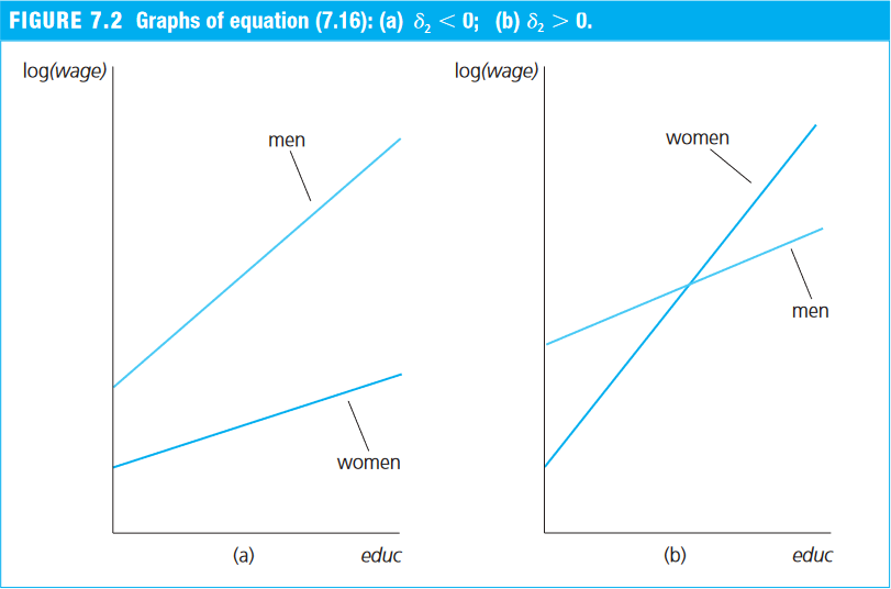
Allowing for Different Slopes
- Section 7.4 of Wooldridge (2006)
- Section 7.5 of Heiss (2020)
- By interacting a continuous variable with a dummy, we allow the slope on the continuous variable to differ across the two categories of the dummy (0 and 1).
Example 7.10: The Log Wage Equation (Wooldridge, 2006)
- Return again to the
wage1dataset from thewooldridgepackage. - Suppose that, in addition to a different intercept, women may also receive a lower return to each additional year of education.
- We therefore include an interaction between the dummy
femaleand years of education (educ):
\begin{align} \log(\text{wage}) = &\beta_0 + \beta_1 \text{female} + \beta_2 \text{educ} + \delta_2 \text{female*educ} \\ &\beta_3 \text{exper} + \beta_4 \text{exper}^2 + \beta_5 \text{tenure} + \beta_6 \text{tenure}^2 + u \end{align} where:
wage: average hourly wagefemale: dummy equal to 1 for women and 0 for meneduc: years of educationfemale*educ: interaction between the dummyfemaleand years of education (educ)exper: years of experience (expersq= years squared)tenure: years with the current employer (tenursq= years squared)
# Load the required dataset
data(wage1, package="wooldridge")

# Estimate the model
reg_7.17 = lm(lwage ~ female + educ + female:educ + exper + expersq + tenure + tenursq,
              data=wage1)
round( summary(reg_7.17)$coef, 4 )
##             Estimate Std. Error t value Pr(>|t|)
## (Intercept)   0.3888     0.1187  3.2759   0.0011
## female       -0.2268     0.1675 -1.3536   0.1764
## educ          0.0824     0.0085  9.7249   0.0000
## exper         0.0293     0.0050  5.8860   0.0000
## expersq      -0.0006     0.0001 -5.3978   0.0000
## tenure        0.0319     0.0069  4.6470   0.0000
## tenursq      -0.0006     0.0002 -2.5089   0.0124
## female:educ  -0.0056     0.0131 -0.4260   0.6703
- An important hypothesis is H$_0:\ \delta_2 = 0$, which tests whether the return to an additional year of education, that is, the slope, differs between women and men.
- The estimates suggest that women’s wages rise about 0.56% less per additional year of education than men’s:
- men’s wages increase by about 8.24% (
educ) for each additional year of schooling; - women’s wages increase by about 7.58% (= 0.0824 - 0.0056) per additional year of schooling.
- men’s wages increase by about 8.24% (
- However, this difference is not statistically significant at the 5% level.