Numerical Optimization
- This section is meant to build intuition for numerical optimization methods.
- We will look at grid search and gradient ascent (descent), which represent two broad families of optimization methods.
Grid Search
- The simplest numerical-optimization method is grid search (discretization).
- Since R cannot handle optimization over an infinite continuum directly, one approach is to discretize the set of possible parameter values within chosen intervals.
- For each candidate parameter combination, we evaluate the objective function. We then choose the combination that maximizes or minimizes that objective.
- The example below considers only one choice parameter, $\theta$. For each point in the interval $[-1, 1]$, we evaluate the objective function:
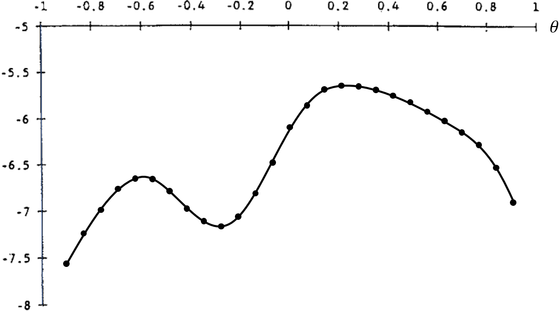
- This method is robust to objective functions with discontinuities and kinks (nondifferentiable points), and it is less sensitive to initial guesses.
- However, it becomes accurate only when many grid points are used, and because the objective function must be evaluated at every point, grid search tends to be computationally expensive.
Gradient Ascent (Descent)
- As the number of model parameters grows, the number of possible parameter combinations rises rapidly, making grid-based search increasingly slow.
- A more efficient way to find the parameter vector that optimizes the objective is to use gradient ascent (descent).
- The goal is to find ${\theta}^{**}$, the parameter value that globally maximizes the objective function.
- Steps to find a maximum:
- Start from an initial parameter value, ${\theta}^0$.
- Compute the derivative and check whether moving “uphill” increases the objective.
- If so, move in the appropriate direction to ${\theta}^1$.
- Repeat steps (2) and (3), moving to ${\theta}^2, {\theta}^3, ...$, until reaching a point where the derivative is zero.
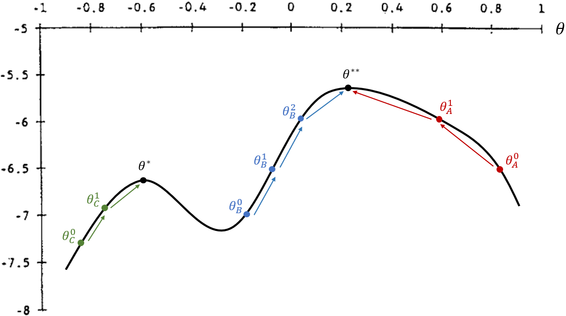
- Notice that this optimization method is sensitive to the initial value and to discontinuities in the objective function.
- In the figure, if the initial guess is ${\theta}^0_A$ or ${\theta}^0_B$, the algorithm reaches the global maximum.
- If the initial guess is ${\theta}^0_C$, it converges to a local maximum at ${\theta}^*$, which is smaller than the global maximum at ${\theta}^{**}$.
- On the other hand, it is more efficient because the objective is evaluated only once per step, and it often yields more precise numerical solutions.
Recovering OLS Through Different Strategies
- In this section, we recover OLS estimates using three strategies: (a) loss-function minimization, (b) maximum likelihood, and (c) the method of moments.
- In each case, we use a different objective to find the two-parameter vector
$ \boldsymbol{\theta} = \{ \beta_0, \beta_1 \} $ that optimizes it. In R, we will call this vector
params.
The mtcars Dataset
We load the dplyr package to manipulate the dataset below.
library(dplyr)
We use data from the 1974 Motor Trend US magazine, which reports fuel consumption and 10 technical characteristics for 32 cars.
In R, this dataset is built in and can be accessed with the code mtcars. The relevant variables here are:
- mpg: miles per gallon
- hp: gross horsepower
We want to estimate the following model: $$ \text{mpg} = \beta_0 + \beta_1 \text{hp} + \varepsilon $$
## OLS regression
reg = lm(formula = mpg ~ hp, data = mtcars)
summary(reg)$coef
##                Estimate Std. Error   t value     Pr(>|t|)
## (Intercept) 30.09886054  1.6339210 18.421246 6.642736e-18
## hp          -0.06822828  0.0101193 -6.742389 1.787835e-07
(a) Loss-Function Minimization
- The loss function used in decision theory here is the sum of squared residuals.
- Under this approach, we look for the estimates $\boldsymbol{\theta} = \{ \hat{\beta}_0,\ \hat{\beta}_1 \}$ that minimize this function.
1. Create a Loss Function That Computes the Sum of Squared Residuals
- The function that computes the sum of squared residuals takes as inputs:
- a vector of possible values for $\boldsymbol{\theta} = \{ \hat{\beta}_0,\ \hat{\beta}_1 \}$;
- a string with the name of the dependent variable;
- a character vector with the names of the regressors;
- a dataset.
resid_quad = function(params, yname, xname, data) {
  # Extract variables from the dataset as vectors
  y = as.matrix(data[yname])
  x = as.matrix(data[xname])

  # Extract parameters from params
  b0 = params[1]
  b1 = params[2]
  sig2 = params[3]

  yhat = b0 + b1 * x # fitted values
  e_hat = y - yhat # residuals = observed - fitted
  sum(e_hat^2)
}
2. Optimization
- We now search for the parameters that minimize the loss function:
- To do so, we use
optim(), which returns the parameters that minimize a function, the numerical equivalent of argmin:
optim(par, fn, gr = NULL, ...,
      method = c("Nelder-Mead", "BFGS", "CG", "L-BFGS-B", "SANN", "Brent"),
      lower = -Inf, upper = Inf,
      control = list(), hessian = FALSE)

par: Initial values for the parameters to be optimized over.
fn: A function to be minimized (or maximized), with first argument the vector of parameters over which minimization is to take place. It should return a scalar result.
method: The method to be used. See ‘Details’. Can be abbreviated.
hessian: Logical. Should a numerically differentiated Hessian matrix be returned?
- We provide as inputs:
- the loss function
resid_quad(); - an initial parameter guess;
- note that optimization can be more or less sensitive to initial values depending on the method used;
- a common neutral starting point is a zero vector such as
c(0, 0, 0); - in Econometrics III, Prof. Laurini recommended starting with the default
"Nelder-Mead"method from zeros and then using those estimates as starting values for"BFGS".
- by default,
hessian = FALSE; set it toTRUEif you want to recover standard errors, t statistics, and p-values from the Hessian.
- the loss function
# Estimate by BFGS
theta_ini = c(0, 0) # initial guess for b0 and b1

fit_ols2 = optim(par=theta_ini, fn=resid_quad,
                 yname="mpg", xname="hp", data=mtcars,
                 method="BFGS", hessian=TRUE)
fit_ols2
## $par
## [1] 30.09886054 -0.06822828
##
## $value
## [1] 447.6743
##
## $counts
## function gradient
##       31        5
##
## $convergence
## [1] 0
##
## $message
## NULL
##
## $hessian
##      [,1]    [,2]
## [1,]   64    9388
## [2,] 9388 1668556
(b) Maximum Likelihood
- ResEcon 703 - Week 6 (University of Massachusetts Amherst)
- Here the objective function is the likelihood function. Unlike the sum of squared residuals, we want to maximize it.
- In this example, we estimate 3 parameters:
Numerical Optimization for Maximum Likelihood
We use optim() again to perform the numerical optimization. The required inputs are:
- initial values for the parameters, $\boldsymbol{\theta}^0 = \{ \beta_0, \beta_1, \sigma^2 \}$;
- a function that takes those parameters as an argument and computes the log-likelihood, $\ln{L(\boldsymbol{\theta})}$.
Since
optim()minimizes the objective function, we need to adapt the log-likelihood output and minimize the negative log-likelihood instead.
The log-likelihood function is given by $$ \ln{L(\beta_0, \beta_1, \sigma^2 | y, x)} = \sum^n_{i=1}{\ln{f(y_i | x_i, \beta_0, \beta_1, \sigma^2)}}, $$
where the conditional distribution of each $y_i$ is
$$ y_i | x_i \sim \mathcal{N}(\beta_0 + \beta_1 x_i, \sigma^2) $$which implies that
$$\varepsilon_i | x_i \sim N(0, \sigma^2)$$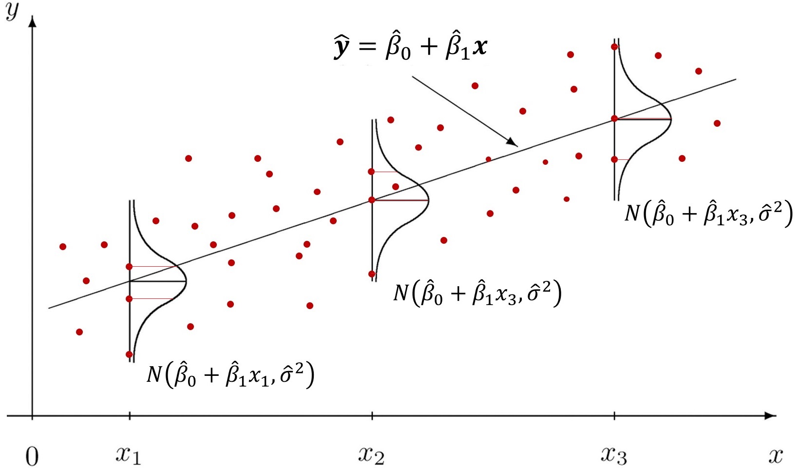
- The figure above shows that for each $x$, we have a fitted value $\hat{y} = \beta_0 + \beta_1 x$, and the disturbances $\varepsilon$ are normally distributed with common variance $\sigma^2$.
Steps to estimate a regression by maximum likelihood:
- Choose initial values for the parameters.
- Compute the fitted values, $\hat{y}$.
- Compute the density for each observation $y_i$, namely $f(y_i | x_i, \beta_0, \beta_1, \sigma^2)$.
- Compute the log-likelihood, $\ln{L(\beta_0, \beta_1, \sigma^2 | y, x)} = \sum^n_{i=1}{\ln{f(y_i | x_i, \beta_0, \beta_1, \sigma^2)}}$.
1. Initial Values for $\beta_0, \beta_1$, and $\sigma^2$
- Unlike OLS, MLE also estimates the variance parameter ( $\sigma^2$).
params = c(30, -0.06, 1)
# (b0, b1 , sig2)
2. Choose the Dataset and Variables
## Initialize objects
yname = "mpg"
xname = "hp"
data = mtcars

# Extract dataset variables as vectors
y = as.matrix(data[yname])
x = as.matrix(data[xname])

# Extract parameter values from params
b0 = params[1]
b1 = params[2]
sig2 = params[3]
3. Compute Fitted Values and Densities
## Compute fitted values of y
yhat = b0 + b1 * x
head(yhat)
##                      hp
## Mazda RX4         23.40
## Mazda RX4 Wag     23.40
## Datsun 710        24.42
## Hornet 4 Drive    23.40
## Hornet Sportabout 19.50
## Valiant           23.70
4. Compute the Densities
$$ f(y_i | x_i, \beta_0, \beta_1, \sigma^2) $$## Compute the pdf for each row
ypdf = dnorm(y, mean = yhat, sd = sqrt(sig2))
head(round(ypdf, 4)) # first density values
##                      mpg
## Mazda RX4         0.0224
## Mazda RX4 Wag     0.0224
## Datsun 710        0.1074
## Hornet 4 Drive    0.0540
## Hornet Sportabout 0.2897
## Valiant           0.0000
sum(ypdf) # likelihood
## [1] 2.447628
prod(ypdf) # likelihood product
## [1] 2.201994e-121
- Now let us combine the objects and inspect their first six rows:
# Combine objects and inspect the first values
tab = cbind(y, x, yhat, round(ypdf, 4)) # round ypdf to 4 digits
colnames(tab) = c("y", "x", "yhat", "ypdf") # rename columns
head(tab)
##                      y   x  yhat   ypdf
## Mazda RX4         21.0 110 23.40 0.0224
## Mazda RX4 Wag     21.0 110 23.40 0.0224
## Datsun 710        22.8  93 24.42 0.1074
## Hornet 4 Drive    21.4 110 23.40 0.0540
## Hornet Sportabout 18.7 175 19.50 0.2897
## Valiant           18.1 105 23.70 0.0000
- As we can see from the combined table and the graphs below, the closer the fitted value is to the observed value for each observation, the higher the associated density/probability.
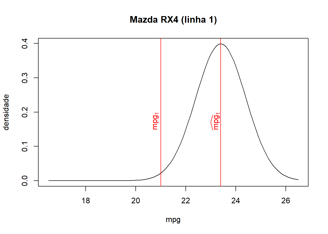
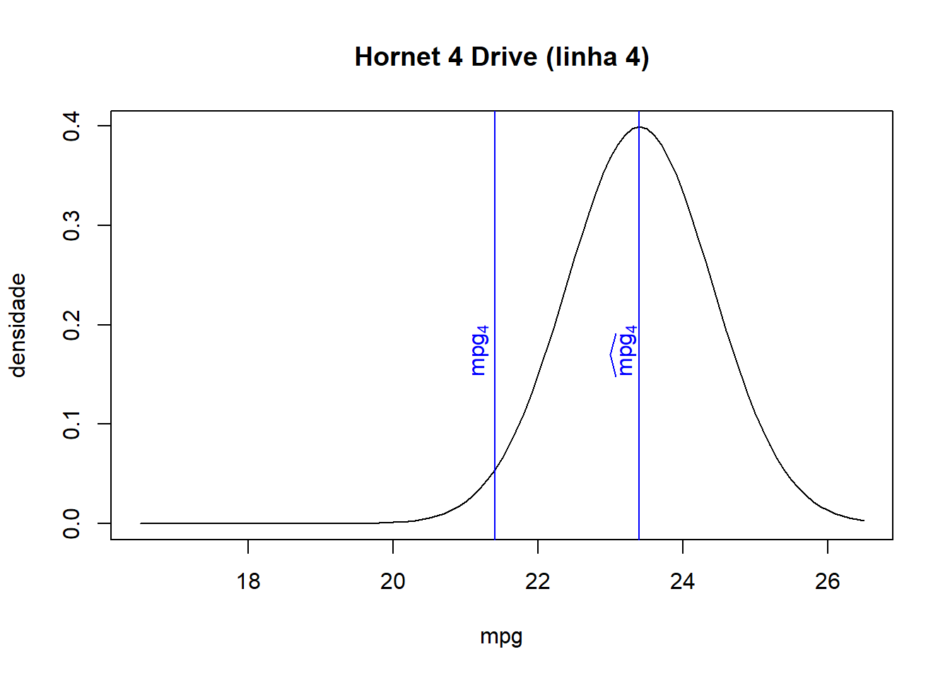
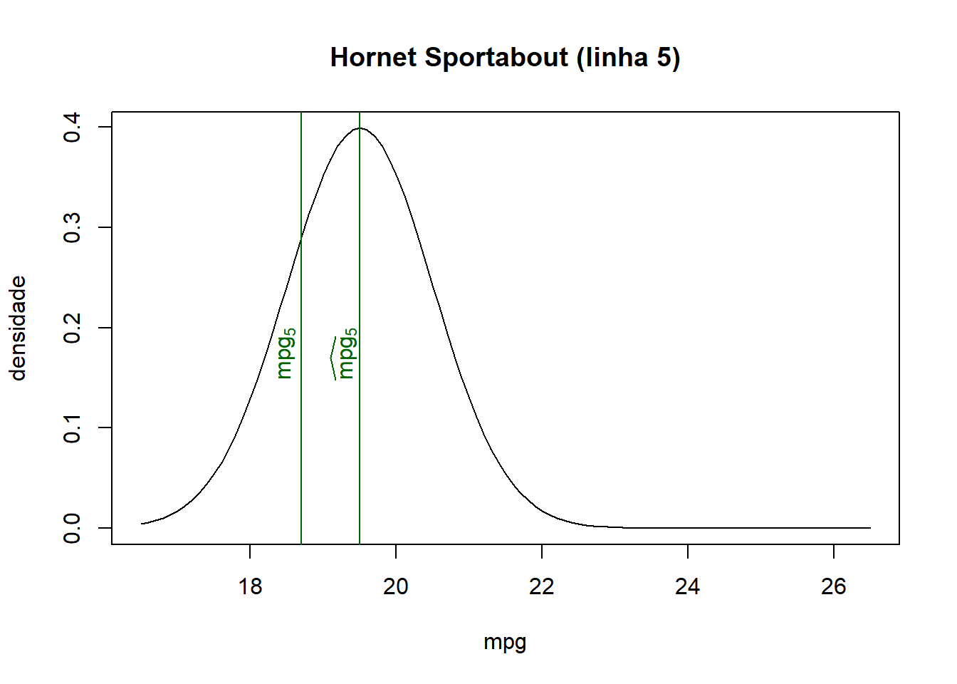
- Therefore, the likelihood, the product of all probabilities, increases when fitted values lie closer to their corresponding observed values.
5. Compute the Log-Likelihood
The log-likelihood is the sum of the log of all probabilities:
$$ \mathcal{l}(\beta_0, \beta_1, \sigma^2) = \sum^{N}_{i=1}{\ln\left[ f(y_i | x_i, \beta_0, \beta_1, \sigma^2) \right]} $$## Compute the log-likelihood
loglik = sum(log(ypdf))
loglik
## [1] -277.8234
6. Create the Log-Likelihood Function
Collecting the previous steps, we can create an R function that evaluates the log-likelihood.
## Create a function to compute the OLS log-likelihood
loglik_lm = function(params, yname, xname, data) {
  # Extract variables from the dataset as vectors
  y = as.matrix(data[yname])
  x = as.matrix(data[xname])

  # Extract parameter values from params
  b0 = params[1]
  b1 = params[2]
  sig2 = params[3]

  ## Compute fitted values of y
  yhat = b0 + b1 * x

  ## Compute the pdf for each row
  ypdf = dnorm(y, mean = yhat, sd = sqrt(sig2))

  ## Compute the log-likelihood
  loglik = sum(log(ypdf))

  ## Return the negative log-likelihood
  -loglik # negative because optim() minimizes and we want to maximize
}
7. Optimization
Now that we have the objective function, we use optim() to minimize
Here we minimize the negative log-likelihood in order to maximize the likelihood itself, since optim() only minimizes.
## Maximize the OLS log-likelihood
mle = optim(par = c(0, 0, 1), fn = loglik_lm,
            yname = "mpg", xname = "hp", data = mtcars,
              method = "BFGS", hessian = TRUE)

## Show optimization results
mle
## $par
## [1] 30.09908613 -0.06822967 13.99015277
##
## $value
## [1] 87.61931
##
## $counts
## function gradient
##       84       28
##
## $convergence
## [1] 0
##
## $message
## NULL
##
## $hessian
##               [,1]         [,2]          [,3]
## [1,]  2.287323e+00 3.355217e+02 -3.520739e-06
## [2,]  3.355217e+02 5.963323e+04  5.199112e-04
## [3,] -3.520739e-06 5.199112e-04  8.174375e-02
## Compute standard errors
# Hessian -> inverse -> diagonal -> square root
mle_se = sqrt( diag( solve(mle$hessian) ) )

# Display estimates and standard errors
cbind(mle$par, mle_se)
##                      mle_se
## [1,] 30.09908613 1.58205585
## [2,] -0.06822967 0.00979809
## [3,] 13.99015277 3.49762080
(c) Method of Moments
Computing Generalized Method of Moments and Generalized Empirical Likelihood with R (Pierre Chausse)
Generalized Method of Moments (GMM) in R - Part 1 (Alfred F. SAM)
To estimate the model by GMM, we need to construct objects related to the following moments:
Notice that these are precisely the moments underlying OLS, since OLS is a special case of GMM. The sample analogs are
$$ \frac{1}{N} \sum^N_{i=1}{\hat{\varepsilon}_i} = 0 \qquad \text{ e } \qquad \frac{1}{N} \sum^N_{i=1}{\hat{\varepsilon}_i.x_i} = 0 $$We can compute both sample moments through a single matrix operation. Consider:
$$ \hat{\boldsymbol{\varepsilon}} = \begin{bmatrix} \varepsilon_1 \\ \varepsilon_2 \\ \vdots \\ \varepsilon_N \end{bmatrix} \qquad \text{e} \qquad \boldsymbol{x} = \begin{bmatrix} x_1 \\ x_2 \\ \vdots \\ x_N \end{bmatrix} $$Join a column of 1s with $\boldsymbol{x}$ and define the matrix: $$ \boldsymbol{X} = \begin{bmatrix} 1 & \varepsilon_1 \\ 1 & \varepsilon_2 \\ \vdots & \vdots \\ 1 & \varepsilon_N \end{bmatrix} $$
Then the matrix multiplication between $\hat{\boldsymbol{\varepsilon}}$ and $\boldsymbol{X}$ gives:
$$ \hat{\boldsymbol{\varepsilon}}' \boldsymbol{X}\ =\ \begin{bmatrix} \varepsilon_1 & \varepsilon_2 & \cdots & \varepsilon_N \end{bmatrix} \begin{bmatrix} 1 & x_1 \\ 1 & x_2 \\ \vdots & \vdots \\ 1 & x_N \end{bmatrix}\ =\ \begin{bmatrix} \frac{1}{N} \sum^N_{i=1}{\hat{\varepsilon}} & \frac{1}{N} \sum^N_{i=1}{\hat{\varepsilon}.x_i} \end{bmatrix} $$The resulting vector contains exactly the sample moments.
Numerical Optimization for GMM
1. Initial Values for $\beta_0$ and $\beta_1$
- Let us create a vector with candidate values for $\beta_0, \beta_1$:
params = c(30, -0.06)
yname = "mpg"
xname = "hp"
data = mtcars
2. Choose the Dataset and Variables
# Extract variables from the dataset as vectors
y = as.matrix(data[yname])
x = as.matrix(data[xname])
X = cbind(1, x)

# Extract parameter values from params
b0 = params[1]
b1 = params[2]
sig2 = params[3]
3. Compute Fitted Values and Residuals
## Fitted values of y
yhat = b0 + b1 * x

## Residuals
e_hat = y - yhat
4. Create the Moment Matrix
- Notice that
$\hat{\boldsymbol{\varepsilon}}' X$ is a vector of sample moments, but the
gmm()function expects a matrix built from the element-by-element multiplication of the residual $\hat{\boldsymbol{\varepsilon}}$ and the covariates $\boldsymbol{X}$ (here: a constant andhp), in the form:
$$ \hat{\boldsymbol{\varepsilon}} \times \boldsymbol{X}\ =\ \begin{bmatrix} \varepsilon_1 \\ \varepsilon_2 \\ \vdots \\ \varepsilon_N \end{bmatrix} \times \begin{bmatrix} 1 & x_1 \\ 1 & x_2 \\ \vdots & \vdots \\ 1 & x_N \end{bmatrix}\ =\ \begin{bmatrix} \varepsilon_1 & \varepsilon_1.x_1 \\ \varepsilon_2 & \varepsilon_2.x_2 \\ \vdots & \vdots \\ \varepsilon_N & \varepsilon_N.x_N \end{bmatrix} $$
For GMM in R, we should not average each column ourselves; the gmm() function will do that internally.
# Moment matrix
m = as.numeric(e_hat) * X
head(m) # first 6 rows
##                              hp
## Mazda RX4         -2.40 -264.00
## Mazda RX4 Wag     -2.40 -264.00
## Datsun 710        -1.62 -150.66
## Hornet 4 Drive    -2.00 -220.00
## Hornet Sportabout -0.80 -140.00
## Valiant           -5.60 -588.00
apply(m, 2, sum) # sum of each column
##                hp
##   -35.46 -6400.62
- Because we multiply the constant term, equal to 1, by the residuals $\varepsilon$, the first column corresponds to the moment $E(\varepsilon)=0$ before taking expectations.
- The remaining columns correspond to moments of the form $E(\varepsilon'X)=0$ for the covariates.
- In GMM, we choose the parameters
$\theta = \{ \beta_0, \beta_1 \}$ so that the sample moments are as close to zero as possible. The
gmm()function handles this numerically, much likeoptim().
5. Create a Function That Returns the Moments
- We now create a function that takes a parameter vector (
params) and data (data) as input, and returns a matrix in which each column represents one moment. - This function bundles together the steps above, which were separated only for exposition.
mom_ols = function(params, list) {
  # In GMM, only one argument besides the parameters is allowed
  # so we pass a list with 3 elements
  yname = list[[1]]
  xname = list[[2]]
  data = list[[3]]

  # Extract variables from the dataset as vectors
  y = as.matrix(data[yname])
  x = as.matrix(data[xname])
  X = cbind(1, x)

  # Extract parameter values from params
  b0 = params[1]
  b1 = params[2]
  sig2 = params[3]

  ## Fitted values of y
  yhat = b0 + b1 * x

  ## Residuals
  e_hat = y - yhat

  ## Moment matrix
  m = as.numeric(e_hat) * X
  m # function output
}
6. Optimization via the gmm() Function
- Like
optim(), thegmm()function takes another function as an argument. - The key difference is that the function supplied to
gmm()returns a matrix rather than a scalar, andgmm()chooses the parameters so that the column means are as close to zero as possible.
library(gmm)
## Loading required package: sandwich
gmm_lm = gmm(g=mom_ols,
             x=list(yname="mpg", xname="hp", data=mtcars), # function arguments
             t0=c(0,0), # initial parameter guess
             wmatrix = "optimal", # weighting matrix
             optfct = "nlminb" # optimization routine
             )

summary(gmm_lm)$coefficients
##             Estimate Std. Error   t value     Pr(>|t|)
## Theta[1] 30.09886038 2.53115147 11.891371 1.312350e-32
## Theta[2] -0.06822828 0.01540378 -4.429319 9.453096e-06