- The econometrics part in R is based on Florian Heiss’s book Using R for Introductory Econometrics (2nd edition, 2020).
- It reproduces in R the content and examples from Wooldridge’s introductory econometrics textbook
- The online version can be read free of charge at: http://www.urfie.net
- There is also a Python version at: http://www.upfie.net
- The datasets used in Wooldridge’s examples can be obtained by installing and loading the
wooldridgepackage:
# install.packages("wooldridge")
library(wooldridge)
Distributions
Probability Distributions in R (Examples): PDF, CDF & Quantile Function (Statistics Globe)
Distribution-related functions follow the structure
<prefix><distribution_name>.There are four main prefixes, each indicating the action to be performed:
d: returns a probability density (pdf)p: returns a cumulative probability from the cumulative distribution function (cdf)q: returns a distribution statistic (quantile) for a given cumulative probabilityr: generates random draws from the distribution
R provides many built-in distributions:
norm: Normalbern: Bernoulli (Rlabpackage)binom: Binomialpois: Poissonchisq: Chi-squared ( $\chi^2$)t: Student’s tf: Funif: Uniformweibull: Weibullgamma: Gammalogis: Logisticexp: Exponential
The main distributions and their associated functions are:
| Distribution | Probability Density | Cumulative Distribution | Quantile |
|---|---|---|---|
| Normal | dnorm(x, mean, sd) | pnorm(q, mean, sd) | qnorm(p, mean, sd) |
| Qui-Quadrado | dchisq(x, df) | pchisq(q, df) | qchisq(p, df) |
| t-Student | dt(x, df) | pt(q, df) | qt(p, df) |
| F | df(x, df1, df2) | pf(q, df1, df2) | qf(p, df1, df2) |
| Binomial | dbinom(x, size, prob) | pbinom(q, size, prob) | qbinom(p, size, prob) |
where x and q are statistics associated with each distribution and p is a probability.
Normal distribution
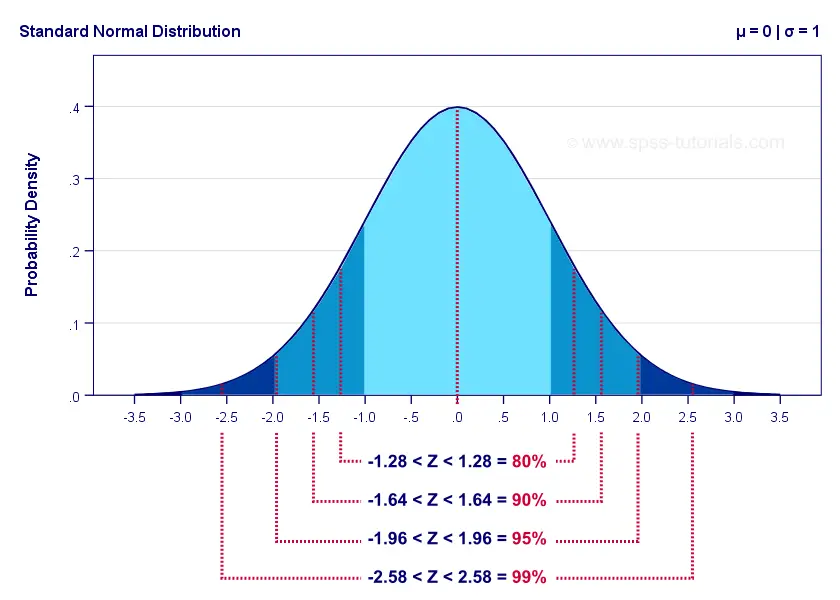
- Consider a standard normal, $N(\mu=0, \sigma=1)$, and the standard scores $Z=-1.96 \text{ and } 1.96$ used in a two-sided confidence interval with significance level of roughly $5\%$:
- [
d]: density from the pdf, given a statistic (standard score):
dnorm(1.96, mean=0, sd=1) # density at a standard score of 1.96
## [1] 0.05844094
dnorm(-1.96, mean=0, sd=1) # density at a standard score of -1.96
## [1] 0.05844094
- [
p]: cumulative probability from the cdf, given a statistic (standard score):
pnorm(1.96, mean=0, sd=1) # cumulative probability up to a standard score of 1.96
## [1] 0.9750021
pnorm(-1.96, mean=0, sd=1) # cumulative probability up to a standard score of -1.96
## [1] 0.0249979
Therefore, the probability that a random variable with a standard normal distribution falls between -1.96 and 1.96 is approximately 95%.
pnorm(1.96, mean=0, sd=1) - pnorm(-1.96, mean=0, sd=1)
## [1] 0.9500042
- [
q]: statistic (standard score) obtained from a quantile:
qnorm(0.975, mean=0, sd=1) # quantile associated with 97.5%
## [1] 1.959964
qnorm(0.025, mean=0, sd=1) # quantile associated with 2.5%
## [1] -1.959964
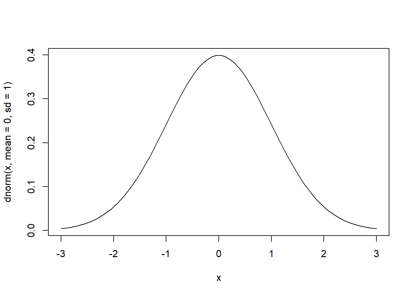
We can draw graphs with curve(function(x), from, to), where we specify a function with an arbitrary x and the lower and upper bounds (from and to):
# pdf of the standard normal over the interval [-3, 3]
curve(dnorm(x, mean=0, sd=1), from=-3, to=3)
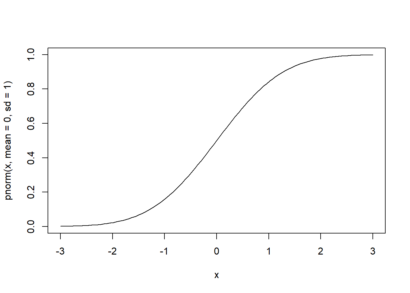
# cdf of the standard normal over the interval [-3, 3]
curve(pnorm(x, mean=0, sd=1), from=-3, to=3)
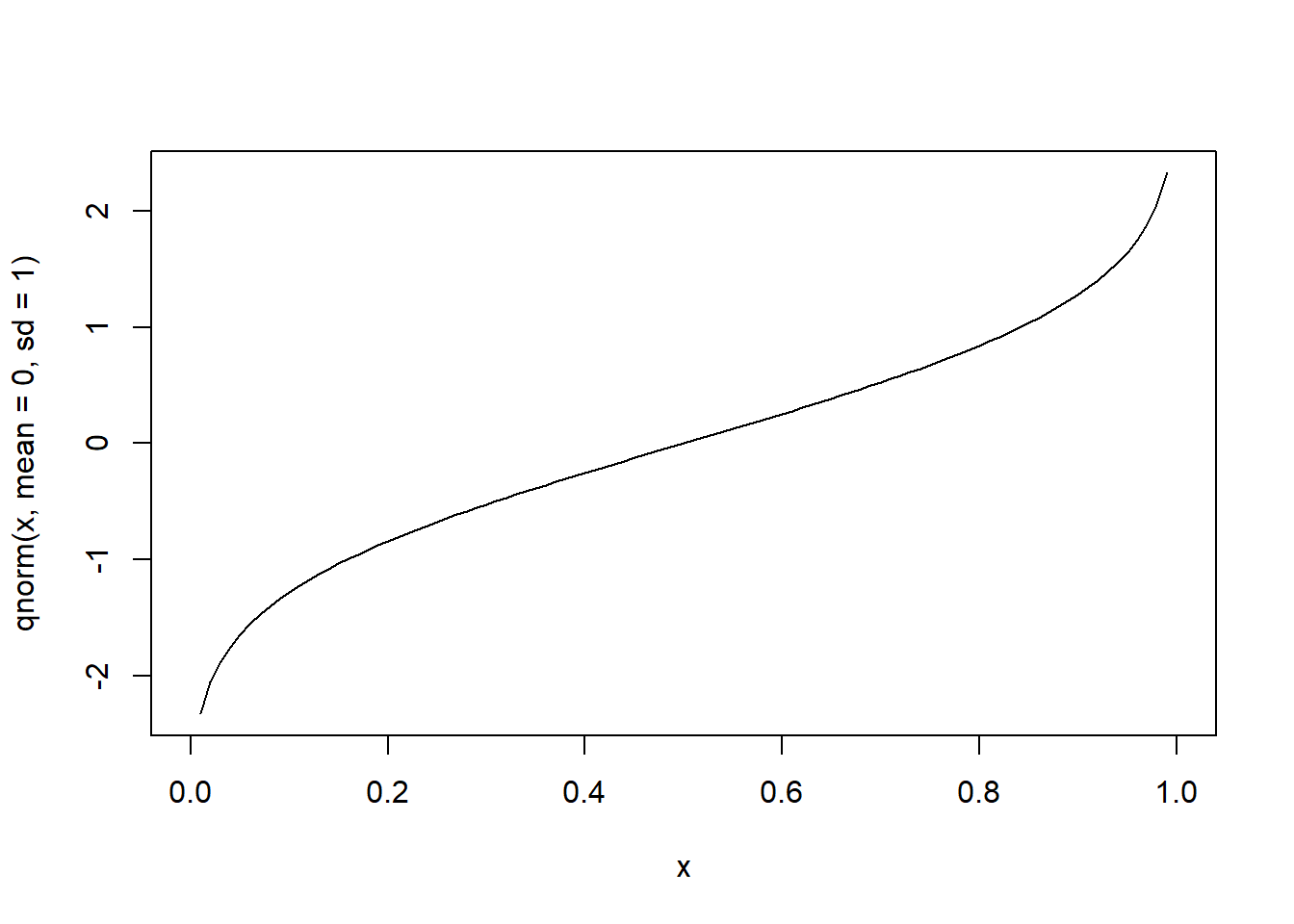
# quantile function of the standard normal over cumulative probabilities in [0, 1]
curve(qnorm(x, mean=0, sd=1), from=0, to=1)
Student’s t distribution
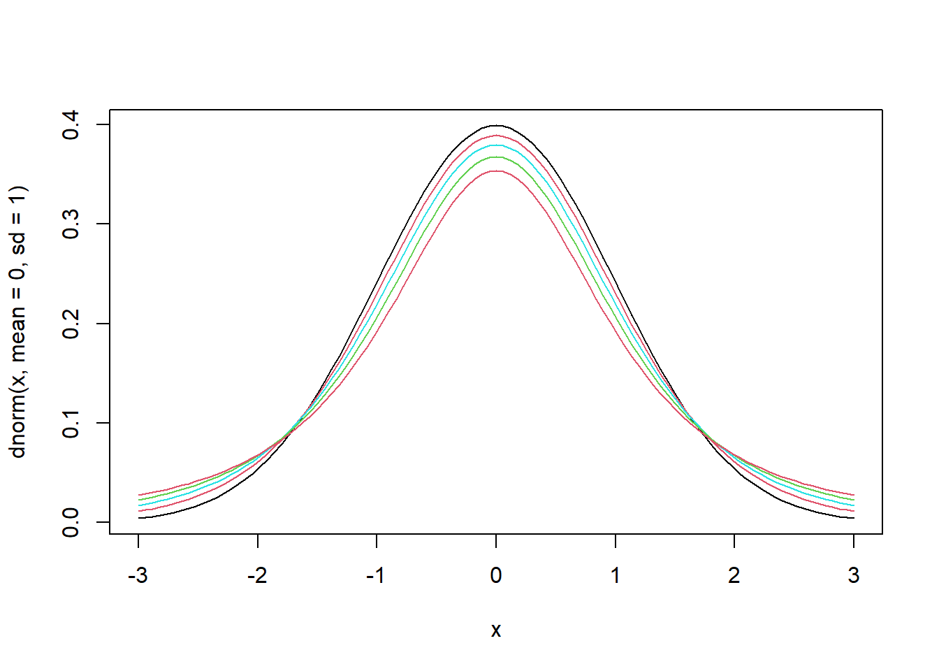
- Let us draw graphs for different degrees of freedom.
- The larger the degrees of freedom, the closer the distribution is to the standard normal.
curve(dnorm(x, mean=0, sd=1), from=-3, to=3, pch=".") # pdf of the standard normal

for (n in c(10, 5, 3, 2)) {
    curve(dt(x, df=n), from=-3, to=3, col=n, add=T) # pdf of Student's t
}
Simulation
Random sampling
- Simulation - Random sampling (John Hopkins/Coursera)
- To draw a sample from a given vector, we use the
sample()function.
sample(x, size, replace = FALSE, prob = NULL)

x: either a vector of one or more elements from which to choose, or a positive integer. See ‘Details.’
n: a positive number, the number of items to choose from.
size: a non-negative integer giving the number of items to choose.
replace: should sampling be with replacement?
prob: a vector of probability weights for obtaining the elements of the vector being sampled.
sample(letters, 5) # sample 5 letters
## [1] "w" "n" "m" "j" "h"
sample(1:10, 4) # sample 4 numbers from 1 to 10
## [1] 5 10 8 6
sample(1:10) # permutation (sample with the same size as the vector)
## [1] 2 10 6 1 5 9 7 3 4 8
sample(1:10, replace = TRUE) # sampling with replacement
## [1] 2 9 9 4 5 1 10 1 4 5
- Notice that, by default,
sample()draws without replacement.
Visualizing the Law of Large Numbers (LLN)
- We can use sampling to simulate repeated rolls of a fair die.
- Let us roll the die once:
sample(1:6, 1) # draw one number from the vector 1:6
## [1] 4
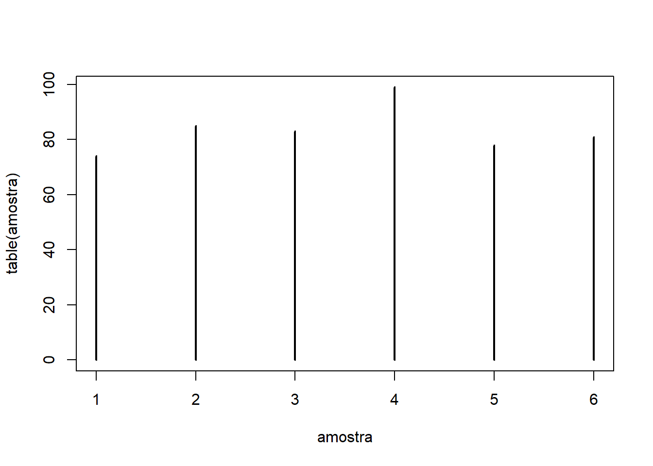
- Now let us roll the die 500 times using
replicate()and inspect the resulting distribution:
sample_draws = replicate(500, expr=sample(1:6, 1))
table(sample_draws) # frequency table of the simulated rolls
## sample_draws
##  1  2  3  4  5  6
## 74 85 83 99 78 81
# Plot
plot(table(sample_draws), type="h")
 - Notice that we cannot use `rep()` for simulation here, because it would draw one number and replicate that same number 500 times.
- Next, let us roll the die twice and compute the average of the two outcomes.
- Notice that we cannot use `rep()` for simulation here, because it would draw one number and replicate that same number 500 times.
- Next, let us roll the die twice and compute the average of the two outcomes.mean(sample(1:6, 2))
## [1] 3.5
- Repeating this procedure 500 times, we obtain:
sample_draws = replicate(500, mean(sample(1:6, 2, replace=T)))
table(sample_draws) # frequency table for the averages of 2 rolls
## sample_draws
##   1 1.5   2 2.5   3 3.5   4 4.5   5 5.5   6
##  10  27  47  61  71  83  61  44  42  33  21
# Plot
plot(table(sample_draws), type="h")
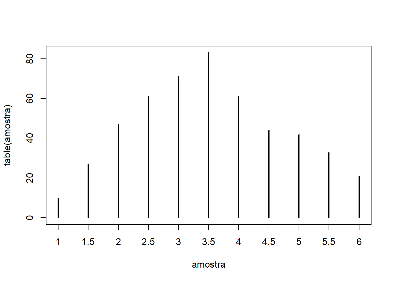
- Notice that, after repeating the experiment 500 times, the average of 2 die rolls already places more mass near the population mean (3.5), although there is still non-negligible density at the extreme values (1 and 6).
- We needed the argument
replace = TRUEso the die outcomes could be drawn with replacement. - If we compute the average of $N=100$ die rolls 500 times, we obtain:
N = 100
sample_draws = replicate(500, mean(sample(1:6, N, replace=T)))

# Plot
plot(table(sample_draws), type="h", xlim=c(1,6))
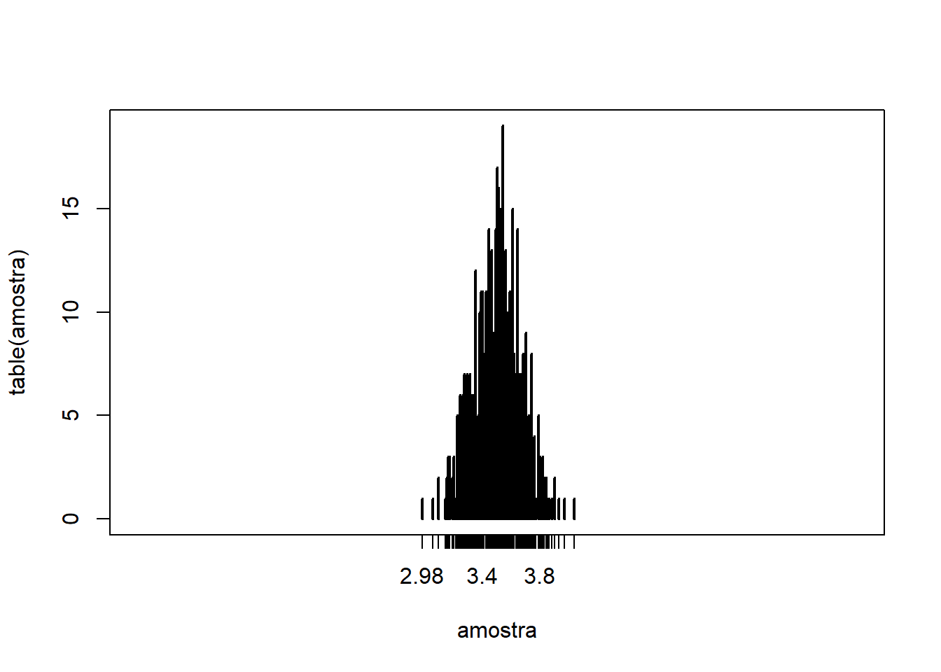
- The larger $N$ becomes, the more tightly the sample means concentrate around the population mean (3.5). At the same time, the probability mass assigned to more distant averages becomes essentially negligible.
Generating random numbers
- To generate random numbers, we use the prefix
rtogether with a distribution name.
rnorm(5) # generate 5 random numbers
## [1] -0.8829037 -0.5396110 0.3302621 0.4478966 -0.5543385
- To reproduce results involving random numbers, we can fix a seed with
set.seed()and supply an integer. The same principle applies tosample().
# setting the seed
set.seed(2022)
rnorm(5)
## [1] 0.9001420 -1.1733458 -0.8974854 -1.4445014 -0.3310136
# without setting the seed
rnorm(5)
## [1] -2.9006290 -1.0592557 0.2779547 0.7494859 0.2415825
# setting the seed again
set.seed(2022)
rnorm(5)
## [1] 0.9001420 -1.1733458 -0.8974854 -1.4445014 -0.3310136
Confidence intervals
- Subsection 1.8.1 of Heiss (2020)
- Appendix C.5 in Wooldridge (2006) derives 95% confidence intervals.
- For a normally distributed population with mean
$\mu$ and variance
$\sigma^2$, the confidence interval with significance level
\(\alpha\)is given by:
$$ \text{IC}\alpha = \left[\bar{y} - C{\alpha/2}.se(\bar{y}),\quad \bar{y} + C_{\alpha/2}.se(\bar{y})\right] \tag{1.2} $$ where:
- $\bar{y}$: sample mean
- $se(\bar{y}) = \frac{s}{\sqrt{n}}$: standard error of $\bar{y}$
- $s$: sample standard deviation
- $n$: sample size
- $C_{\alpha/2}$: the critical value corresponding to the
$(1-\alpha/2)$ quantile of the
$t_{n-1}$ distribution
- For example, when $\alpha = 5\%$, we use the 97.5% quantile ( $= 1 - 5\%/2$)
- When the number of degrees of freedom is large, the t distribution approaches the standard normal. Therefore, for a 95% confidence interval, the critical value is approximately $C_{2.5\%} \approx 1.96$
Example C.2: Effect of corporate training subsidies on worker productivity (Wooldridge, 2006)
- Holzer, Block, Cheatham, and Knott (1993) studied the effects of corporate training subsidies on worker productivity.
- Their outcome variable is the “scrap rate”, that is, the number of discarded items per 100 produced units.
- Between 1987 and 1988, 20 firms received corporate training, and we want to know whether this affected the scrap rate, that is, whether the difference between the two yearly means is statistically significant (different from 0).
- Let us begin by creating vectors with the scrap rates for the 20 firms in 1987 (SR87) and 1988 (SR88):
SR87 = c(10, 1, 6, .45, 1.25, 1.3, 1.06, 3, 8.18, 1.67, .98,
         1, .45, 5.03, 8, 9, 18, .28, 7, 3.97)
SR88 = c(3, 1, 5, .5, 1.54, 1.5, .8, 2, .67, 1.17, .51, .5,
         .61, 6.7, 4, 7, 19, .2, 5, 3.83)
- Create the vector of scrap-rate changes and compute the relevant statistics:
Change = SR88 - SR87 # vector of changes
n = length(Change) # number of firms / length of the change vector
avgChange = mean(Change) # mean of the change vector
sdChange = sd(Change) # standard deviation of the change vector
- Compute the standard error and the critical value for a 95% confidence interval:
se = sdChange / sqrt(n) # standard error
CV = qt(.975, n-1) # critical value for a 95% confidence interval
- Finally, compute the confidence interval using equation (1.2):
c(avgChange - CV*se, avgChange + CV*se) # lower and upper limits of the interval
## [1] -2.27803369 -0.03096631
# we could also write the interval more compactly:
avgChange + CV * c(-se, se)
## [1] -2.27803369 -0.03096631
- Since 0 lies outside the 95% confidence interval, we conclude that the scrap rate changed, and that the effect is statistically significant and negative.
t test and p-values
Appendix C.6 of Wooldridge (2006)
The t statistic for testing a hypothesis about a normally distributed random variable $y$ with mean $\bar{y}$ is given by equation C.35 in Wooldridge (2006). Under the null hypothesis $H_0: \bar{y} = \mu_0$, $$ t = \frac{\bar{y} - \mu_0}{se(\bar{y})}. \tag{1.3} $$
To reject the null hypothesis, the absolute value of the t statistic must exceed the critical value at a given significance level $\alpha$.
For example, at the $\alpha = 5\%$ significance level and with a large sample, so that the t distribution is close to the standard normal, we reject the null if $$ |t| \ge 1.96 \approx \text{critical value at the 5% significance level} $$
The advantage of using the p-value is its convenience, since we can compare it directly with the significance level.
For two-sided t tests, the p-value is given by equation C.42 in Wooldridge (2006): $$ p = 2.Pr(T_{n-1} > |t|) = 2.[1 - F_{t_{n-1}}(|t|)] $$ where $F_{t_{n-1}}(\cdot)$ is the cdf of the $t_{n-1}$ distribution.
- We reject the null hypothesis if the p-value is smaller than the significance level $\alpha$.
Example C.6: Effect of corporate training subsidies on worker productivity (Wooldridge, 2006)
- Continuation of Example C.2
- Considering a two-sided test, we can calculate the t statistic:
# t statistic for H0: mu = 0
t = (avgChange - 0) / se
print(paste0("t statistic = ", abs(t), " > ", CV, " = critical value"))
## [1] "t statistic = 2.15071100397349 > 2.09302405440831 = critical value"
- Since the t statistic is greater than the critical value, we reject $H_0$ at the 5% significance level.
- Equivalently, we can compute the p-value:
p = 2 * (1 - pt(abs(t), n-1))
print(paste0("p-value = ", p, " < 0.05 = significance level"))
## [1] "p-value = 0.0445812529367844 < 0.05 = significance level"
- Since the p-value is smaller than $\alpha = 5\%$, we reject $H_0$.
Computation with t.test()
t.test(x, y = NULL,
       alternative = c("two.sided", "less", "greater"),
       mu = 0, paired = FALSE, var.equal = FALSE,
       conf.level = 0.95, ...)

x: (non-empty) numeric vector of data values.
alternative: a character string specifying the alternative hypothesis, must be one of "two.sided" (default), "greater" or "less". You can specify just the initial letter.
mu: a number indicating the true value of the mean (or difference in means if you are performing a two sample test).
conf.level: confidence level of the interval.
- Notice that we supply a vector of values in the argument
x. By default, the function performs a two-sided test of $H_0$ under the null that the true mean is zero, together with a 95% confidence interval. - Returning to Examples C.2 and C.6, we obtain:
testresults = t.test(Change)
testresults
##
## 	One Sample t-test
##
## data:  Change
## t = -2.1507, df = 19, p-value = 0.04458
## alternative hypothesis: true mean is not equal to 0
## 95 percent confidence interval:
##  -2.27803369 -0.03096631
## sample estimates:
## mean of x
##   -1.1545
- The test-results object contains the following components:
names(testresults)
##  [1] "statistic"   "parameter"   "p.value"     "conf.int"    "estimate"
##  [6] "null.value"  "stderr"      "alternative" "method"      "data.name"
- For example, we can access the p-value with:
testresults$p.value
## [1] 0.04458125