Data Manipulation in R

“Between 30% to 80% of the data analysis task is spent on cleaning and understanding the data.” (Dasu & Johnson, 2003)

In this section, we use the starwars dataset from the dplyr package to review the main tools for data manipulation in R.

library(dplyr)

# We will refer to the starwars dataset as sw
sw = starwars

# Drop the last three columns to simplify the examples.
# These columns are lists.
sw[, c("films", "vehicles", "starships")] = NULL

The `base` package

In this section, we manipulate datasets using the functions that are loaded by default in R.

Summarizing data

Basic functions

Summarizing data (John Hopkins/Coursera)
We will inspect:
- the dataset dimensions with dim()
- the first six rows with head()
- the last six rows with tail()

dim(sw) # dataset size (rows x columns)

head(sw) # first six rows

tail(sw) # last six rows

With str(), we can inspect the structure of the dataset:
- all variables (columns)
- the class of each variable
- a sample of the observations

str(sw)

To generate a summary for all variables, we can use summary(). For numeric variables, the function reports quantiles, the mean, and the number of missing values.

summary(sw)

For logical, text, or categorical variables, summary() is usually less informative. In those cases, it is often useful to build a frequency table with table() and then turn it into percentages with prop.table(table()).

table(sw$hair_color) # counts

prop.table(table(sw$hair_color)) # percentages

We can also build a cross-tabulation by including more than one variable inside table():

table(sw$hair_color, sw$gender)

The `apply` family

The apply family provides compact ways to repeat operations:

apply(): applies a function to the rows or columns of a matrix or array
lapply(): applies a function to each element of a list
sapply(): similar to lapply(), but tries to simplify the output

The `apply()` function

Loop functions - apply (John Hopkins/Coursera)
apply() is commonly used to evaluate a function over the rows or columns of a matrix.
It is not necessarily faster than writing an explicit loop, but it is concise and readable.

apply(X, MARGIN, FUN, ...)

X: an array, including a matrix.
MARGIN: a vector giving the dimensions over which the function will be applied.
FUN: the function to be applied.
...: optional arguments passed to FUN.

x = matrix(1:20, 5, 4)
x

apply(x, 1, mean) # row means

apply(x, 2, mean) # column means

There are built-in functions that reproduce these operations directly:
- rowSums = apply(x, 1, sum)
- rowMeans = apply(x, 1, mean)
- colSums = apply(x, 2, sum)
- colMeans = apply(x, 2, mean)

The `lapply()` function

Loop functions - lapply (John Hopkins/Coursera)
lapply() takes three main inputs: a list, a function, and optional additional arguments.

lapply(X, FUN, ...)

X: a vector (atomic or list) or an expression object.
FUN: the function to be applied to each element of X.
...: optional arguments passed to FUN.

lapply() applies a function to each element of the list.
A data frame is a special kind of list whose elements are its columns.

lapply(sw, mean, na.rm = TRUE)

Notice that non-numeric variables return NA, and the third argument above is an argument of mean().
We can also inspect the unique values of each variable by combining lapply() with unique():

lapply(sw, unique)

A particularly useful application is counting the number of missing values in each column. Because is.na(sw) returns a matrix, we can combine it with apply():

head(is.na(sw)) # first rows after applying is.na()

class(is.na(sw)) # object type

apply(is.na(sw), 2, sum) # sum TRUE/FALSE by column

The `sapply()` function

sapply() is similar to lapply(), but it tries to simplify the result whenever possible.
If each list element returns an object of the same length, sapply() often returns a vector or matrix instead of a list.

sapply(sw, mean, na.rm = TRUE)

Filtering rows

Subsetting and sorting (John Hopkins/Coursera)

# logical vector for blond hair
sw$hair_color == "blond"

# extract rows with blond hair
sw[sw$hair_color == "blond", ]

We can use logical expressions to filter observations. For example, suppose we want characters with blond hair and non-missing hair_color:

sw[sw$hair_color == "blond" & !is.na(sw$hair_color), ]

To avoid repeating the dataset name before each variable, we can use with():

with(sw,
     sw[hair_color == "blond" & !is.na(hair_color), ]
)

We could also extract observations with blond or white hair:

# extract rows where hair is blond or white
sw[sw$hair_color == "blond" | sw$hair_color == "white", ]

We can also check whether values belong to a given vector with %in%, which is equivalent to applying == to several values at once:

sw$hair_color %in% c("blond", "white") # TRUE/FALSE for blond or white hair

sw = sw[sw$hair_color %in% c("blond", "white"), ]
head(sw)

Reordering rows

Subsetting and sorting (John Hopkins/Coursera)
We can use sort() to order a vector in ascending order (default) or descending order.

sort(sw$height) # ascending order

sort(sw$height, decreasing = TRUE) # descending order

sort() is not appropriate for reordering a full data frame, because it returns only a vector.
To reorder data frames, we use order(), which returns the row indices from the smallest values to the largest.

order(sw$height) # row indices in ascending order of height

sw = sw[order(sw$height), ] # reorder the data frame
head(sw)

Selecting columns

We can select columns with [,] by passing a vector of names or indices to keep.

# Select the first three columns
head(sw[, c("name", "height", "mass")])

# Select the first six columns
sw = sw[, 1:6]
head(sw)

Renaming columns

We can rename variables with names() or colnames() by assigning a new vector of names.

names(sw) # current variable names

# Remove underscores
names(sw)[4] = "haircolor" # change one name
names(sw)[5:6] = c("skincolor", "eyecolor") # change two names
names(sw)

Modifying columns

To modify a variable, we can assign a vector of the same length using $.

sw$height = sw$height / 100 # convert cm to meters

If we assign a scalar, R repeats it for all observations:

sw$const = 1

We can also create new variables:

sw$BMI = sw$mass / sw$height^2 # body mass index
head(sw)

Common variable transformations (John Hopkins/Coursera)

abs(sw$BMI[1:4]) # absolute value

sqrt(sw$BMI[1:4]) # square root

ceiling(sw$BMI[1:4]) # round up

floor(sw$BMI[1:4]) # round down

round(sw$BMI[1:4], digits = 1) # one decimal place

cos(sw$BMI[1:4]) # cosine

sin(sw$BMI[1:4]) # sine

log(sw$BMI[1:4]) # natural logarithm

log10(sw$BMI[1:4]) # base-10 logarithm

exp(sw$BMI[1:4]) # exponential

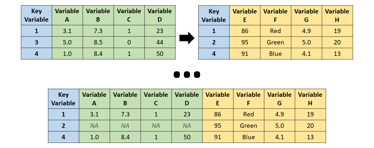
Merging datasets

Merging data (John Hopkins/Coursera)
Joining (Merging) Data (David E. Caughlin)
A merge matches cases, that is, rows or observations, across two datasets using one or more key variables:

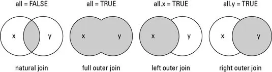
We use the merge() function for that purpose:

merge(x, y, by = intersect(names(x), names(y)),
      by.x = by, by.y = by, all = FALSE, all.x = all, all.y = all,
      suffixes = c(".x", ".y"), ...)

x, y: data frames, or objects that can be coerced into data frames.
by, by.x, by.y: columns used for merging.
all: shorthand for setting both all.x and all.y.
all.x: keep all rows from x.
all.y: keep all rows from y.
suffixes: suffixes used when non-key variables share the same name.

Let us create two datasets where some individuals appear in one dataset but not in the other:

# Extract smaller data frames from the original starwars dataset
bd1 = starwars[1:6, c(1, 3, 11)]
bd1

bd2 = starwars[c(2, 4, 7:10), c(1:2, 6)]
bd2

There are 12 unique characters across the two datasets, but only "C-3PO" and "Darth Vader" appear in both.
To check which columns share the same name, we can combine intersect() with names() or colnames():

intersect(names(bd1), names(bd2))

If we do not specify the key variable, merge() uses all columns with matching names.

Inner join

merge(bd1, bd2, all = FALSE)

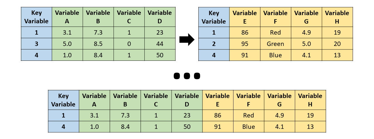
Full join

merge(bd1, bd2, all = TRUE)

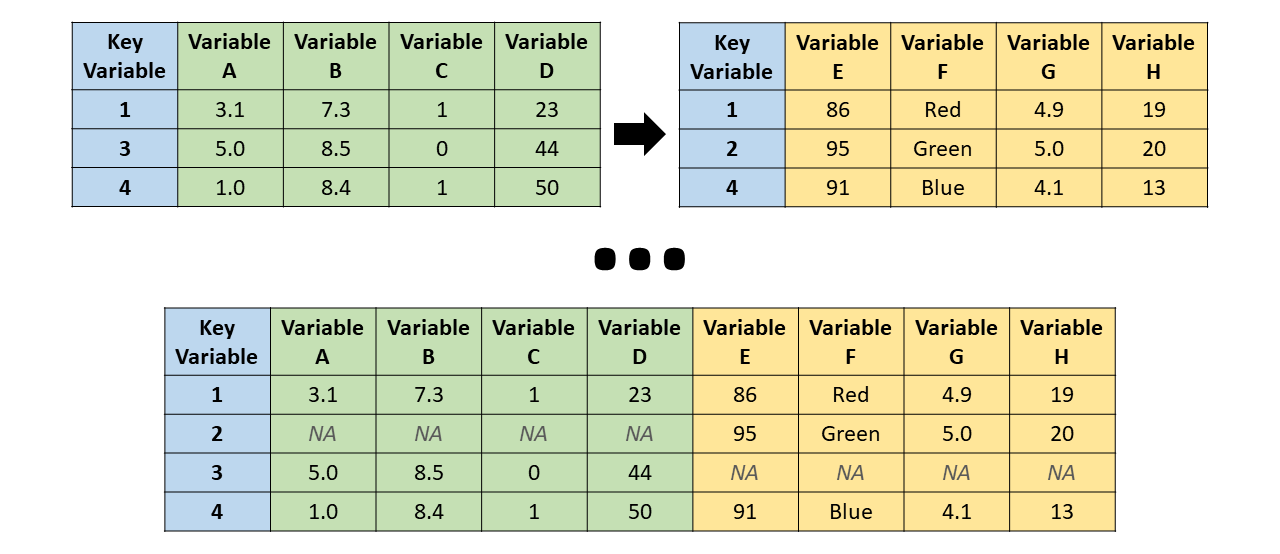
Left join

merge(bd1, bd2, all.x = TRUE)

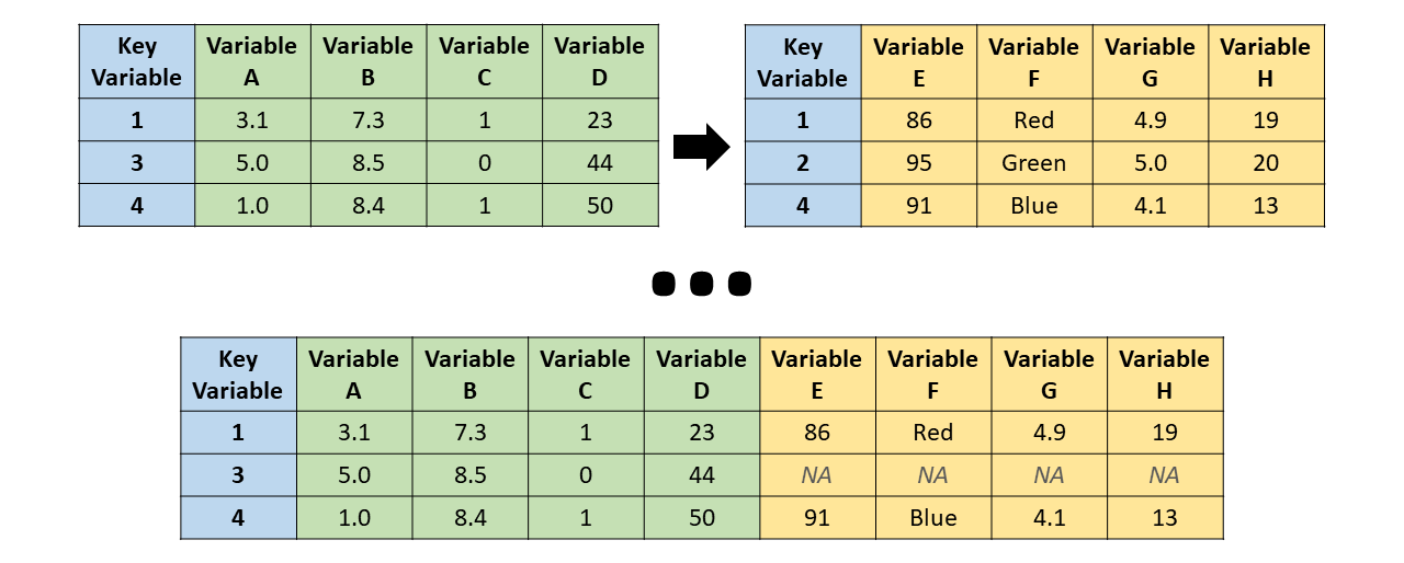
Right join

merge(bd1, bd2, all.y = TRUE)

The `dplyr` package

Vignette - Introduction to dplyr
The dplyr package makes data manipulation easier through simple and computationally efficient functions.
These functions can be grouped into three categories:
- Columns:
  - select(): selects or drops data-frame columns
  - rename(): changes column names
  - mutate(): creates or modifies column values
- Rows:
  - filter(): selects rows according to column values
  - arrange(): reorders the rows
- Groups of rows:
  - summarise(): collapses each group into a single row
  - group_by(): creates grouped data
In this subsection, we continue using the Star Wars dataset.
You will notice that, when these functions are applied, the data frame is turned into a tibble, which is a more efficient format for tabular data but works very similarly to a standard data frame.

library("dplyr") # load package

head(starwars) # inspect the first rows of the dataset included in the package

Filter rows with `filter()`

Selects a subset of rows from a data frame.

filter(.data, ...)

.data: a data frame or tibble.
...: logical expressions defined in terms of the variables in .data.

starwars1 = filter(starwars, species == "Human", height >= 100)
starwars1

# Equivalent to:
starwars[starwars$species == "Human" & starwars$height >= 100, ]

Reorder rows with `arrange()`

Reorders the rows according to one or more column names.

arrange(.data, ..., .by_group = FALSE)

.data: a data frame or tibble.
...: variables, or functions of variables. Use desc() for descending order.

If more than one variable is provided, the data are first ordered by the first variable and ties are broken using the second.

starwars2 = arrange(starwars1, height, desc(mass))
starwars2

Select columns with `select()`

Selects the columns of interest.

select(.data, ...)

...: variables in a data frame.

We can list the variables we want to keep, select ranges with var1:var2, or drop variables with -var.

starwars3 = select(starwars2, name:eye_color, sex:species)
# equivalent: select(starwars2, -birth_year, -c(films:starships))
starwars3

head(select(starwars, ends_with("color")))

head(select(starwars, starts_with("s")))

Notice that select() may not work properly if the MASS package is attached. If that happens, detach MASS in the Packages pane or run detach("package:MASS", unload = TRUE).

Rename columns with `rename()`

Renames columns using new_name = old_name.

rename(.data, ...)

.data: a data frame or tibble.
...: use new_name = old_name to rename selected variables.

starwars4 = rename(
  starwars3,
  haircolor = hair_color,
  skincolor = skin_color,
  eyecolor = eye_color
)
starwars4

Modify/Add columns with `mutate()`

Modifies an existing column.
Creates a new column if it does not exist.

mutate(.data, ...)

.data: a data frame or tibble.
...: name-value pairs defining the output columns.

starwars5 = mutate(
  starwars4,
  height = height / 100, # convert cm to meters
  BMI = mass / height^2,
  dummy = 1 # a scalar is recycled to all rows
)
starwars5 = select(starwars5, BMI, dummy, everything())
starwars5

The pipe operator `%>%`

Notice that all previous dplyr functions take the dataset as their first argument.
The pipe operator %>% passes the object on the left-hand side into the first argument of the function on the right-hand side.

filter(starwars, species == "Droid") # without the pipe

starwars %>% filter(species == "Droid") # with the pipe

When we use the pipe operator, the dataset should not be written again as the first argument because %>% passes it automatically.
Also note that, from filter() through mutate(), we have been accumulating transformations in new data frames. The last object, starwars5, is the result of applying the full sequence of changes to the original starwars dataset.

starwars1 = filter(starwars, species == "Human", height >= 100)
starwars2 = arrange(starwars1, height, desc(mass))
starwars3 = select(starwars2, name:eye_color, sex:species)
starwars4 = rename(
  starwars3,
  haircolor = hair_color,
  skincolor = skin_color,
  eyecolor = eye_color
)
starwars5 = mutate(
  starwars4,
  height = height / 100,
  BMI = mass / height^2,
  dummy = 1
)
starwars5 = select(starwars5, BMI, dummy, everything())
starwars5

By chaining the same commands with %>%, we can write the full workflow as a single pipeline:

starwars_pipe = starwars %>%
  filter(species == "Human", height >= 100) %>%
  arrange(height, desc(mass)) %>%
  select(name:eye_color, sex:species) %>%
  rename(
    haircolor = hair_color,
    skincolor = skin_color,
    eyecolor = eye_color
  ) %>%
  mutate(
    height = height / 100,
    BMI = mass / height^2,
    dummy = 1
  ) %>%
  select(BMI, dummy, everything())
starwars_pipe

all(starwars_pipe == starwars5, na.rm = TRUE)

Summarize with `summarise()`

We can use summarise() to compute statistics for one or more variables:

starwars %>% summarise(
  n_obs = n(),
  mean_height = mean(height, na.rm = TRUE),
  mean_mass = mean(mass, na.rm = TRUE)
)

In the example above, we simply computed the sample size and the mean height and mass for the full sample.

Group data with `group_by()`

Unlike the other dplyr functions shown so far, group_by() does not change the contents of the data frame. It only turns the data into a grouped dataset according to the categories of one or more variables.

grouped_sw = starwars %>% group_by(sex)
class(grouped_sw)

head(starwars)

head(grouped_sw)

group_by() is useful whenever the next operation depends on multiple rows. As an illustration, let us create a column with the mean value of mass across all observations:

starwars %>%
  mutate(mean_mass = mean(mass, na.rm = TRUE)) %>%
  select(mean_mass, sex, everything()) %>%
  head(10)

Notice that all values of mean_mass are identical. We now group by sex before computing the mean:

starwars %>%
  group_by(sex) %>%
  mutate(mean_mass = mean(mass, na.rm = TRUE)) %>%
  ungroup() %>%
  select(mean_mass, sex, everything()) %>%
  head(10)

This is useful in many economics applications in which we work with group-level variables, for example household-level statistics attached to individual observations.

Avoid mistakes: whenever you use group_by(), remember to run ungroup() after the grouped operation if the next commands should not remain grouped.

Grouped summaries with `group_by()` and `summarise()`

summarise() becomes especially useful when combined with group_by(), because it lets us compute statistics at the group level:

summary_sw = starwars %>%
  group_by(sex) %>%
  summarise(
    n_obs = n(),
    mean_height = mean(height, na.rm = TRUE),
    mean_mass = mean(mass, na.rm = TRUE)
  )
summary_sw

class(summary_sw)

After summarise(), the resulting data frame is no longer grouped, so ungroup() is not needed in this case.
We can also group by more than one variable:

starwars %>%
  group_by(sex, hair_color) %>%
  summarise(
    n_obs = n(),
    mean_height = mean(height, na.rm = TRUE),
    mean_mass = mean(mass, na.rm = TRUE)
  )

To group continuous variables, we first need to define intervals with cut():

cut(x, ...)

x: a numeric vector that will be turned into a factor by cutting it into intervals.
breaks: either a vector of cut points or a single integer giving the number of intervals.

# breaks supplied as an integer = desired number of groups
starwars %>%
  group_by(cut(birth_year, breaks = 5)) %>%
  summarise(
    n_obs = n(),
    mean_height = mean(height, na.rm = TRUE)
  )

# breaks supplied as a vector = explicit cut points
starwars %>%
  group_by(birth_year = cut(birth_year, breaks = c(0, 40, 90, 200, 900))) %>%
  summarise(
    n_obs = n(),
    mean_height = mean(height, na.rm = TRUE)
  )

Notice that we wrote birth_year = cut(birth_year, ...) so the grouped column keeps the name birth_year.

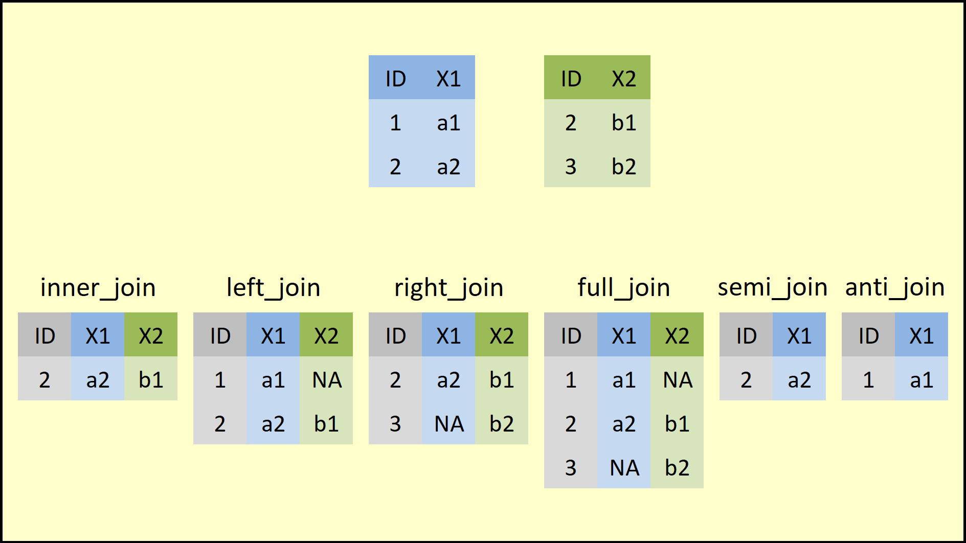
Join datasets with `_join_` functions

Earlier we saw that merge() combines datasets through key variables.
The dplyr package provides a family of _join_ functions that accomplish the same task with a cleaner interface:

The common ingredients are:
- x: dataset 1
- y: dataset 2
- by: vector of key variables
- suffix: suffixes used when non-key variables share the same name
As an example, we use subsets of the starwars dataset:

bd1 = starwars[1:6, c(1, 3, 11)]
bd2 = starwars[c(2, 4, 7:10), c(1:2, 6)]
bd1
bd2

There are 12 unique characters across the two datasets, but only "C-3PO" and "Darth Vader" appear in both.
inner_join(): keeps only IDs present in both datasets

inner_join(bd1, bd2, by = "name")

full_join(): keeps all IDs, even if they appear in only one dataset

full_join(bd1, bd2, by = "name")

left_join(): keeps the IDs present in dataset 1, supplied as x

left_join(bd1, bd2, by = "name")

right_join(): keeps the IDs present in dataset 2, supplied as y

right_join(bd1, bd2, by = "name")

Proceed to Data Visualization

The base package

Summarizing data

Basic functions

The apply family

The apply() function

The lapply() function

The sapply() function

Filtering rows

Reordering rows

Selecting columns

Renaming columns

Modifying columns

Merging datasets

Inner join

Full join

Left join

Right join

The dplyr package

Filter rows with filter()

Reorder rows with arrange()

Select columns with select()

Rename columns with rename()

Modify/Add columns with mutate()

The pipe operator %>%

Summarize with summarise()

Group data with group_by()

Grouped summaries with group_by() and summarise()

Join datasets with _join_ functions

The `base` package

The `apply` family

The `apply()` function

The `lapply()` function

The `sapply()` function

The `dplyr` package

Filter rows with `filter()`

Reorder rows with `arrange()`

Select columns with `select()`

Rename columns with `rename()`

Modify/Add columns with `mutate()`

The pipe operator `%>%`

Summarize with `summarise()`

Group data with `group_by()`

Grouped summaries with `group_by()` and `summarise()`

Join datasets with `_join_` functions