Panel Data Manipulation
- In the applications we are studying, the dataset is typically required to be
- in long format: for each individual, we have one row per period;
- balanced: the sample size is $N \times T$, with $N$ individuals and $T$ periods; and
- properly ordered by individual and then by time.
- In many empirical applications, the information is released as a collection of cross-sectional datasets, so we first need to build the panel structure.
- In R, there are at least two ways to do this:
- stack the datasets and keep only the individuals who appear in every period; or
- perform an inner join by individual and then convert the data from wide to long.
- As an example, we will use PNAD Continua, which is released quarterly and can be handled with the
PNADcIBGEpackage. - The data can be imported with
read_pnadc(microdata, input_txt), which requires downloading both the microdata files and the text file containing the variable metadata (input_txt) from the IBGE FTP:
# install.packages("PNADcIBGE")
# install.packages("dplyr")
library(PNADcIBGE)
library(dplyr)
- The compressed
.zipfile is about 12% of the size of the uncompressed.txtfile (133 MB $\times$ 1.08 GB). To avoid keeping the.txtfile permanently on the computer, we can useunz()to extract it temporarily:
# Unzipping the PNADc files and loading them into R
pnad_012021 = read_pnadc(unz("PNADC_012021_20220224.zip", "PNADC_012021.txt"),
                         input_txt = "input_PNADC_trimestral.txt")

pnad_022021 = read_pnadc(unz("PNADC_022021_20220224.zip", "PNADC_022021.txt"),
                         input_txt = "input_PNADC_trimestral.txt")
- To identify an individual in the PNAD data, IBGE uses the following key variables:
- UPA: Primary Sampling Unit / State code (2) + Sequential Number (6) + Check Digit (1)
- V1008: Household number (01 to 14)
- V1014: Panel/sample group (01 to 99)
- V2003: Within-household order number (01 to 30)
- Researchers at Ipea (Teixeira Junior et al., 2020) add a few time-invariant key variables to make this identifier more robust:
- V2007: Sex
- V2008/V20081/V20082: Date of birth (day/month/year)
- In addition, we will keep a few more variables:
- time-invariant:
- UF: State
- time-varying:
- V2009: Age (in years)
- VD4020: Effective monthly labor income for people aged 14 or older
- time-invariant:
# List of variables used in the example
lista_var = c("Trimestre", "UPA", "V1008", "V1014", "V2003", "V2007", "V2008",
              "V20081", "V20082", "UF", "V2009", "VD4020")

# Selecting and renaming variables, and keeping only people aged 14 or older
pnad_1 = pnad_012021 %>% select(all_of(lista_var)) %>%
    rename(DOMIC = V1008, PAINEL = V1014, ORDEM = V2003, SEXO = V2007,
           DIA_NASC = V2008, MES_NASC = V20081, ANO_NASC = V20082,
           IDADE = V2009, RENDA = VD4020) %>%
    filter(IDADE >= 14)

pnad_2 = pnad_022021 %>% select(all_of(lista_var)) %>%
    rename(DOMIC = V1008, PAINEL = V1014, ORDEM = V2003, SEXO = V2007,
           DIA_NASC = V2008, MES_NASC = V20081, ANO_NASC = V20082,
           IDADE = V2009, RENDA = VD4020) %>%
    filter(IDADE >= 14)
Stacking datasets and keeping individuals observed in every period
- First, we stack the two datasets with
rbind(). They must have the same number of columns, and the corresponding columns must share the same class (character, numeric, etc.):
pnad_bind = rbind(pnad_1, pnad_2)
head(pnad_bind)
## # A tibble: 6 × 12
##   Trimestre UPA     DOMIC PAINEL ORDEM SEXO  DIA_N…¹ MES_N…² ANO_N…³ UF    IDADE
##   <chr>     <chr>   <chr> <chr>  <chr> <chr> <chr>   <chr>   <chr>   <chr> <dbl>
## 1 1         110000… 01    08     01    2     16      05      1981    11       39
## 2 1         110000… 01    08     02    2     12      06      2000    11       20
## 3 1         110000… 01    08     03    2     15      05      2004    11       16
## 4 1         110000… 01    08     04    1     26      07      1947    11       73
## 5 1         110000… 01    08     05    2     15      08      1961    11       59
## 6 1         110000… 02    08     01    2     11      07      1983    11       37
## # … with 1 more variable: RENDA <dbl>, and abbreviated variable names
## #   ¹​DIA_NASC, ²​MES_NASC, ³​ANO_NASC
- Note that the 2nd observation does not correspond to the same person as the 1st row. We therefore create an
IDvariable by concatenating all key variables and then reorder the data by that identifier and by quarter:
pnad_bind = pnad_bind %>% mutate(
    ID = paste0(UPA, DOMIC, PAINEL, ORDEM, SEXO, DIA_NASC, MES_NASC, ANO_NASC)
    ) %>% select(ID, everything()) %>% # reorder variables so ID comes first
    arrange(ID, Trimestre)
head(pnad_bind, 10)
## # A tibble: 10 × 13
## ID Trime…¹ UPA DOMIC PAINEL ORDEM SEXO DIA_N…² MES_N…³ ANO_N…â´ UF
## <chr> <chr> <chr> <chr> <chr> <chr> <chr> <chr> <chr> <chr> <chr>
## 1 1100000… 1 1100… 01 08 01 2 16 05 1981 11
## 2 1100000… 1 1100… 01 08 02 2 12 06 2000 11
## 3 1100000… 1 1100… 01 08 03 2 15 05 2004 11
## 4 1100000… 1 1100… 01 08 04 1 26 07 1947 11
## 5 1100000… 1 1100… 01 08 05 2 15 08 1961 11
## 6 1100000… 1 1100… 02 08 01 2 11 07 1983 11
## 7 1100000… 2 1100… 02 08 01 2 11 07 1983 11
## 8 1100000… 1 1100… 02 08 02 1 99 99 9999 11
## 9 1100000… 2 1100… 02 08 02 1 99 99 9999 11
## 10 1100000… 1 1100… 03 08 01 2 09 03 1976 11
## # … with 2 more variables: IDADE <dbl>, RENDA <dbl>, and abbreviated variable
## # names ¹​Trimestre, ²​DIA_NASC, ³​MES_NASC, â´​ANO_NASC
- Observe that the panel is not balanced: not every individual appears in both quarters. So we first create an auxiliary object that counts how many times each
IDappears inpnad_bind:
cont_ID = pnad_bind %>% group_by(ID) %>% summarise(cont = n())
head(cont_ID, 10)
## # A tibble: 10 × 2
##    ID                        cont
##    <chr>                    <int>
##  1 110000016010801216051981     1
##  2 110000016010802212062000     1
##  3 110000016010803215052004     1
##  4 110000016010804126071947     1
##  5 110000016010805215081961     1
##  6 110000016020801211071983     2
##  7 110000016020802199999999     2
##  8 110000016030801209031976     2
##  9 110000016030802103092000     2
## 10 110000016030804118091954     2
- In
cont_ID, we keep only the cases that appear exactly twice:
cont_ID = cont_ID %>% filter(cont == 2)
head(cont_ID, 10)
## # A tibble: 10 × 2
##    ID                        cont
##    <chr>                    <int>
##  1 110000016020801211071983     2
##  2 110000016020802199999999     2
##  3 110000016030801209031976     2
##  4 110000016030802103092000     2
##  5 110000016030804118091954     2
##  6 110000016040801105081969     2
##  7 110000016040802215011976     2
##  8 110000016040803110071994     2
##  9 110000016040804217051997     2
## 10 110000016050801105071965     2
- Back in
pnad_bind, we filter the sample to keep only IDs that are present incont_ID$ID:
pnad_bind = pnad_bind %>% filter(ID %in% cont_ID$ID)
head(pnad_bind)
## # A tibble: 6 × 13
## ID Trime…¹ UPA DOMIC PAINEL ORDEM SEXO DIA_N…² MES_N…³ ANO_N…â´ UF
## <chr> <chr> <chr> <chr> <chr> <chr> <chr> <chr> <chr> <chr> <chr>
## 1 11000001… 1 1100… 02 08 01 2 11 07 1983 11
## 2 11000001… 2 1100… 02 08 01 2 11 07 1983 11
## 3 11000001… 1 1100… 02 08 02 1 99 99 9999 11
## 4 11000001… 2 1100… 02 08 02 1 99 99 9999 11
## 5 11000001… 1 1100… 03 08 01 2 09 03 1976 11
## 6 11000001… 2 1100… 03 08 01 2 09 03 1976 11
## # … with 2 more variables: IDADE <dbl>, RENDA <dbl>, and abbreviated variable
## # names ¹​Trimestre, ²​DIA_NASC, ³​MES_NASC, â´​ANO_NASC
N = pnad_bind$ID %>% unique() %>% length() # number of unique individuals
T = pnad_bind$Trimestre %>% unique() %>% length() # number of unique quarters
paste0("N = ", N, ", T = ", T, ", NT = ", N*T)
## [1] "N = 174468, T = 2, NT = 348936"
Joining the datasets and converting from wide to long
- Now we join the datasets with
inner_join(), which keeps only the individuals who appear in both files:
pnad_joined = inner_join(pnad_1, pnad_2,
                         by=c("UPA", "DOMIC", "PAINEL", "ORDEM", "SEXO",
                              "DIA_NASC", "MES_NASC", "ANO_NASC"),
                         suffix=c("_1", "_2")) # avoid using . as a separator
colnames(pnad_joined) # column names
##  [1] "Trimestre_1" "UPA"         "DOMIC"       "PAINEL"      "ORDEM"
##  [6] "SEXO"        "DIA_NASC"    "MES_NASC"    "ANO_NASC"    "UF_1"
## [11] "IDADE_1"     "RENDA_1"     "Trimestre_2" "UF_2"        "IDADE_2"
## [16] "RENDA_2"
dim(pnad_joined) # dataset dimensions
## [1] 174468 16
- The joined data are now in wide format (one row per individual), and the information for the 2 periods (the first and second quarters of 2021) appears in separate columns:
- The suffixes were added to duplicate columns present in both datasets but not listed in
by. - The time-invariant variable UF was duplicated as well, so it makes sense to include it among the key variables.
- The suffixes were added to duplicate columns present in both datasets but not listed in
pnad_joined = inner_join(pnad_1, pnad_2,
                         by=c("UPA", "DOMIC", "PAINEL", "ORDEM", "SEXO",
                              "DIA_NASC", "MES_NASC", "ANO_NASC", "UF"),
                         suffix=c("_1", "_2")) # avoid using . as a separator
colnames(pnad_joined) # column names
##  [1] "Trimestre_1" "UPA"         "DOMIC"       "PAINEL"      "ORDEM"
##  [6] "SEXO"        "DIA_NASC"    "MES_NASC"    "ANO_NASC"    "UF"
## [11] "IDADE_1"     "RENDA_1"     "Trimestre_2" "IDADE_2"     "RENDA_2"
dim(pnad_joined) # dataset dimensions
## [1] 174468 15
- We now have a single UF column, and the number of observations remains unchanged because sampled households did not actually switch states between these quarters.
- If the number of rows had changed, that would indicate that some supposedly time-invariant observations differed across periods and were therefore dropped.
- We can also remove the columns
Trimestre_1andTrimestre_2:
pnad_joined = pnad_joined %>% select(-Trimestre_1, -Trimestre_2)
- Since the dataset is still in wide format, we now convert it to long format.
Converting from wide to long with tidyr
To reshape data between wide and long formats, we will use
tidyrand the functionspivot_longer(),pivot_wider(), andseparate().
library(tidyr)
pivot_longer(): converts several columns into two columns, one for names and one for values (it increases the number of rows and decreases the number of columns)
pivot_longer(
  data,
  cols,
  names_to = "name",
  values_to = "value"
  ...
)
pivot_wider(): converts unique values of a variable into separate columns (it increases the number of columns and decreases the number of rows)
pivot_wider(
  data,
  names_from = name,
  values_from = value,
  values_fill = NULL
  ...
)
separate(): splits one column into multiple columns using a separator character
separate(
  data,
  col,
  into,
  sep = "[^[:alnum:]]+"
  ...
)
- First, we reshape the time-varying columns (with suffixes
_1or_2) into two columns:
library(tidyr)
pnad_joined2 = pnad_joined %>%
    pivot_longer(
        cols = c(ends_with("_1"), ends_with("_2") ),
        names_to = "VAR_TRI", # new column that stores former column names
        values_to = "VALUE" # new column that stores the reshaped values
    )
head(pnad_joined2)
## # A tibble: 6 × 11
##   UPA       DOMIC PAINEL ORDEM SEXO  DIA_N…¹ MES_N…² ANO_N…³ UF    VAR_TRI VALUE
##   <chr>     <chr> <chr>  <chr> <chr> <chr>   <chr>   <chr>   <chr> <chr>   <dbl>
## 1 110000016 02    08     01    2     11      07      1983    11    IDADE_1    37
## 2 110000016 02    08     01    2     11      07      1983    11    RENDA_1    NA
## 3 110000016 02    08     01    2     11      07      1983    11    IDADE_2    37
## 4 110000016 02    08     01    2     11      07      1983    11    RENDA_2    NA
## 5 110000016 02    08     02    1     99      99      9999    11    IDADE_1    31
## 6 110000016 02    08     02    1     99      99      9999    11    RENDA_1    NA
## # … with abbreviated variable names ¹​DIA_NASC, ²​MES_NASC, ³​ANO_NASC
- Instead of having 2 rows per individual, we now have 4 because there are 2 time-varying variables.
- We therefore need to move half of those rows back into columns. We use
separate()to split VAR_TRI (with 4 unique values: IDADE_1, IDADE_2, RENDA_1, and RENDA_2) into 2 columns: VAR (with 2 unique values: IDADE and RENDA) and TRI (with 2 unique values: 1 and 2).
pnad_joined3 = pnad_joined2[1:100,] %>%
    separate(
        col = "VAR_TRI",
        into = c("VAR", "TRI"), # names of the new columns
        sep = "_" # separator used in VAR_TRI
    )
head(pnad_joined3)
## # A tibble: 6 × 12
##   UPA   DOMIC PAINEL ORDEM SEXO  DIA_N…¹ MES_N…² ANO_N…³ UF    VAR   TRI   VALUE
##   <chr> <chr> <chr>  <chr> <chr> <chr>   <chr>   <chr>   <chr> <chr> <chr> <dbl>
## 1 1100… 02    08     01    2     11      07      1983    11    IDADE 1        37
## 2 1100… 02    08     01    2     11      07      1983    11    RENDA 1        NA
## 3 1100… 02    08     01    2     11      07      1983    11    IDADE 2        37
## 4 1100… 02    08     01    2     11      07      1983    11    RENDA 2        NA
## 5 1100… 02    08     02    1     99      99      9999    11    IDADE 1        31
## 6 1100… 02    08     02    1     99      99      9999    11    RENDA 1        NA
## # … with abbreviated variable names ¹​DIA_NASC, ²​MES_NASC, ³​ANO_NASC
- Finally, we convert the VAR column (with the 2 unique values IDADE and RENDA) into 2 separate columns:
pnad_joined4 = pnad_joined3 %>%
    pivot_wider(
        names_from = "VAR",
        values_from = "VALUE"
    )
pnad_joined4 %>% select(TRI, everything()) %>% head(20)
## # A tibble: 20 × 12
##    TRI   UPA       DOMIC PAINEL ORDEM SEXO  DIA_NASC MES_N…¹ ANO_N…² UF    IDADE
##    <chr> <chr>     <chr> <chr>  <chr> <chr> <chr>    <chr>   <chr>   <chr> <dbl>
##  1 1     110000016 02    08     01    2     11       07      1983    11       37
##  2 2     110000016 02    08     01    2     11       07      1983    11       37
##  3 1     110000016 02    08     02    1     99       99      9999    11       31
##  4 2     110000016 02    08     02    1     99       99      9999    11       31
##  5 1     110000016 03    08     01    2     09       03      1976    11       44
##  6 2     110000016 03    08     01    2     09       03      1976    11       45
##  7 1     110000016 03    08     02    1     03       09      2000    11       20
##  8 2     110000016 03    08     02    1     03       09      2000    11       20
##  9 1     110000016 03    08     04    1     18       09      1954    11       66
## 10 2     110000016 03    08     04    1     18       09      1954    11       66
## 11 1     110000016 04    08     01    1     05       08      1969    11       51
## 12 2     110000016 04    08     01    1     05       08      1969    11       51
## 13 1     110000016 04    08     02    2     15       01      1976    11       44
## 14 2     110000016 04    08     02    2     15       01      1976    11       45
## 15 1     110000016 04    08     03    1     10       07      1994    11       26
## 16 2     110000016 04    08     03    1     10       07      1994    11       26
## 17 1     110000016 04    08     04    2     17       05      1997    11       23
## 18 2     110000016 04    08     04    2     17       05      1997    11       23
## 19 1     110000016 05    08     01    1     05       07      1965    11       55
## 20 2     110000016 05    08     01    1     05       07      1965    11       55
## # … with 1 more variable: RENDA <dbl>, and abbreviated variable names
## #   ¹​MES_NASC, ²​ANO_NASC
Extra: Creating dummies with pivot_wider()
- First, create a column of 1s.
- Then use
pivot_wider(), specifying the categorical variable and the column of 1s, while replacing missing values with zero (fill = 0):
dummies_sexo = pnad_1 %>% mutate(const = 1) %>% # creating a column of 1s
    pivot_wider(names_from = SEXO,
                values_from = const,
                values_fill = 0)
head(dummies_sexo)
## # A tibble: 6 × 13
##   Trimestre UPA     DOMIC PAINEL ORDEM DIA_N…¹ MES_N…² ANO_N…³ UF    IDADE RENDA
##   <chr>     <chr>   <chr> <chr>  <chr> <chr>   <chr>   <chr>   <chr> <dbl> <dbl>
## 1 1         110000… 01    08     01    16      05      1981    11       39  1045
## 2 1         110000… 01    08     02    12      06      2000    11       20  1045
## 3 1         110000… 01    08     03    15      05      2004    11       16    NA
## 4 1         110000… 01    08     04    26      07      1947    11       73    NA
## 5 1         110000… 01    08     05    15      08      1961    11       59    NA
## 6 1         110000… 02    08     01    11      07      1983    11       37    NA
## # … with 2 more variables: `2` <dbl>, `1` <dbl>, and abbreviated variable names
## #   ¹​DIA_NASC, ²​MES_NASC, ³​ANO_NASC
Another example 1: wide to long
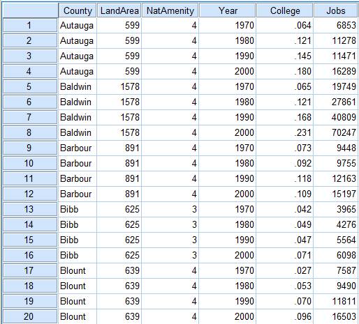
- The dataset below contains information for 5 counties, including land area, the share of adults with college education, and the number of jobs in 4 different years:
bd_counties = data.frame(
    county = c("Autauga", "Baldwin", "Barbour", "Bibb", "Blount"),
    area = c(599, 1578, 891, 625, 639),
    college_1970 = c(.064, .065, .073, .042, .027),
    college_1980 = c(.121, .121, .092, .049, .053),
    college_1990 = c(.145, .168, .118, .047, .070),
    college_2000 = c(.180, .231, .109, .071, .096),
    jobs_1970 = c(6853, 19749, 9448, 3965, 7587),
    jobs_1980 = c(11278, 27861, 9755, 4276, 9490),
    jobs_1990 = c(11471, 40809, 12163, 5564, 11811),
    jobs_2000 = c(16289, 70247, 15197, 6098, 16503)
)
bd_counties
##    county area college_1970 college_1980 college_1990 college_2000 jobs_1970
## 1 Autauga  599        0.064        0.121        0.145        0.180      6853
## 2 Baldwin 1578        0.065        0.121        0.168        0.231     19749
## 3 Barbour  891        0.073        0.092        0.118        0.109      9448
## 4    Bibb  625        0.042        0.049        0.047        0.071      3965
## 5  Blount  639        0.027        0.053        0.070        0.096      7587
##   jobs_1980 jobs_1990 jobs_2000
## 1     11278     11471     16289
## 2     27861     40809     70247
## 3      9755     12163     15197
## 4      4276      5564      6098
## 5      9490     11811     16503
- We want to reshape the dataset so that each county has 4 rows, one for each year: 1970, 1980, 1990, or 2000. The final structure should therefore have 5 columns: county, year, area, college, and jobs. We begin by stacking the columns whose names start with
college_andjobs_usingpivot_longer():
bd_counties2 = bd_counties %>%
    pivot_longer(
        cols = c( starts_with("college_"), starts_with("jobs_") ),
        names_to = "var_year", # new column that stores the former column names
        values_to = "value" # new column that stores the reshaped values
    )
head(bd_counties2, 10)
## # A tibble: 10 × 4
##    county   area var_year         value
##    <chr>   <dbl> <chr>            <dbl>
##  1 Autauga   599 college_1970     0.064
##  2 Autauga   599 college_1980     0.121
##  3 Autauga   599 college_1990     0.145
##  4 Autauga   599 college_2000     0.18
##  5 Autauga   599 jobs_1970     6853
##  6 Autauga   599 jobs_1980    11278
##  7 Autauga   599 jobs_1990    11471
##  8 Autauga   599 jobs_2000    16289
##  9 Baldwin  1578 college_1970     0.065
## 10 Baldwin  1578 college_1980     0.121
- For each county, there are now two rows per year because there are 2 time-varying variables (college and jobs). We remove this duplication by using
separate()to splitvar_yearinto two columns, which we callvarandyear:
bd_counties3 = bd_counties2 %>%
    separate(
        col = "var_year",
        into = c("var", "year"), # names of the new columns
        sep = "_" # separator used in the original column "var_year"
    )
head(bd_counties3, 10)
## # A tibble: 10 × 5
##    county   area var     year      value
##    <chr>   <dbl> <chr>   <chr>     <dbl>
##  1 Autauga   599 college 1970      0.064
##  2 Autauga   599 college 1980      0.121
##  3 Autauga   599 college 1990      0.145
##  4 Autauga   599 college 2000      0.18
##  5 Autauga   599 jobs    1970   6853
##  6 Autauga   599 jobs    1980  11278
##  7 Autauga   599 jobs    1990  11471
##  8 Autauga   599 jobs    2000  16289
##  9 Baldwin  1578 college 1970      0.065
## 10 Baldwin  1578 college 1980      0.121
- Next, we transform the
varcolumn into 2 columns (collegeandjobs) withpivot_wider():
bd_counties4 = bd_counties3 %>%
    pivot_wider(
        names_from = "var",
        values_from = "value"
    )
bd_counties4 %>% select(county, year, everything()) %>% head(10)
## # A tibble: 10 × 5
##    county  year   area college  jobs
##    <chr>   <chr> <dbl>   <dbl> <dbl>
##  1 Autauga 1970    599   0.064  6853
##  2 Autauga 1980    599   0.121 11278
##  3 Autauga 1990    599   0.145 11471
##  4 Autauga 2000    599   0.18  16289
##  5 Baldwin 1970   1578   0.065 19749
##  6 Baldwin 1980   1578   0.121 27861
##  7 Baldwin 1990   1578   0.168 40809
##  8 Baldwin 2000   1578   0.231 70247
##  9 Barbour 1970    891   0.073  9448
## 10 Barbour 1980    891   0.092  9755
- If there were only one time-varying variable,
pivot_wider()would not be necessary because there would already be one row per county-year observation.
Another example 2: long to wide
- We now use the
TravelModedataset from theAERpackage, which contains 840 observations in which 210 individuals choose among 4 travel modes: car, air, train, or bus. - Each of the 210 individuals appears in 4 rows, one for each travel mode.
- The dataset contains variables specific to
- the individual (individual, income, and size), which are repeated across the 4 rows where that person appears; and
- the choice occasion (choice, wait, vcost, travel, and gcost), which vary with the travel mode.
data("TravelMode", package = "AER")
head(TravelMode, 8)
##   individual  mode choice wait vcost travel gcost income size
## 1          1   air     no   69    59    100    70     35    1
## 2          1 train     no   34    31    372    71     35    1
## 3          1   bus     no   35    25    417    70     35    1
## 4          1   car    yes    0    10    180    30     35    1
## 5          2   air     no   64    58     68    68     30    2
## 6          2 train     no   44    31    354    84     30    2
## 7          2   bus     no   53    25    399    85     30    2
## 8          2   car    yes    0    11    255    50     30    2
- We now reshape the dataset so that each individual appears in only one row, dropping the mode column and generating several columns for each possible travel mode.
TravelMode2 = TravelMode %>%
    pivot_wider(
        names_from = "mode",
        values_from = c("choice":"gcost") # mode-specific variables
    )
head(TravelMode2)
## # A tibble: 6 × 23
## individ…¹ income size choic…² choic…³ choic…â´ choic…âµ wait_…ⶠwait_…â· wait_…â¸
## <fct> <int> <int> <fct> <fct> <fct> <fct> <int> <int> <int>
## 1 1 35 1 no no no yes 69 34 35
## 2 2 30 2 no no no yes 64 44 53
## 3 3 40 1 no no no yes 69 34 35
## 4 4 70 3 no no no yes 64 44 53
## 5 5 45 2 no no no yes 64 44 53
## 6 6 20 1 no yes no no 69 40 35
## # … with 13 more variables: wait_car <int>, vcost_air <int>, vcost_train <int>,
## # vcost_bus <int>, vcost_car <int>, travel_air <int>, travel_train <int>,
## # travel_bus <int>, travel_car <int>, gcost_air <int>, gcost_train <int>,
## # gcost_bus <int>, gcost_car <int>, and abbreviated variable names
## # ¹​individual, ²​choice_air, ³​choice_train, â´​choice_bus, âµ​choice_car,
## # â¶​wait_air, â·​wait_train, â¸​wait_bus
- For each travel mode, 5 columns were created, corresponding to the 5 mode-specific variables. In total, 6 columns were removed (mode plus the 5 mode-specific variables) and 20 columns were created instead (4 modes $\times$ 5 mode-specific variables).
- In some econometric applications, such as multinomial logit, we want a single column indicating the chosen alternative. We therefore create a
choicecolumn that records the selected option (air, train, bus, or car) and then drop the 4 columns whose names start withchoice_:
TravelMode3 = TravelMode2 %>%
    mutate(
        choice = case_when(
            choice_air == "yes" ~ "air",
            choice_train == "yes" ~ "train",
            choice_bus == "yes" ~ "bus",
            choice_car == "yes" ~ "car"
        )
    ) %>% select(individual, choice,
                 starts_with("wait_"), starts_with("vcost_"),
                 starts_with("travel_"), starts_with("gcost_")
                 )

TravelMode3 %>% head(10)
## # A tibble: 10 × 18
## individual choice wait_air wait_train wait_…¹ wait_…² vcost…³ vcost…â´ vcost…âµ
## <fct> <chr> <int> <int> <int> <int> <int> <int> <int>
## 1 1 car 69 34 35 0 59 31 25
## 2 2 car 64 44 53 0 58 31 25
## 3 3 car 69 34 35 0 115 98 53
## 4 4 car 64 44 53 0 49 26 21
## 5 5 car 64 44 53 0 60 32 26
## 6 6 train 69 40 35 0 59 20 13
## 7 7 air 45 34 35 0 148 111 66
## 8 8 car 69 34 35 0 121 52 50
## 9 9 car 69 34 35 0 59 31 25
## 10 10 car 69 34 35 0 58 31 25
## # … with 9 more variables: vcost_car <int>, travel_air <int>,
## # travel_train <int>, travel_bus <int>, travel_car <int>, gcost_air <int>,
## # gcost_train <int>, gcost_bus <int>, gcost_car <int>, and abbreviated
## # variable names ¹​wait_bus, ²​wait_car, ³​vcost_air, â´​vcost_train, âµ​vcost_bus