- Sections 8.2 and 8.3 of Heiss (2020)
- Sections 5.5 and 7.1 to 7.4 of Davidson and MacKinnon (1999)
- Sections 4.2.3 and 4.2.4 of Wooldridge
Error variance-covariance matrix
Recall that the error variance-covariance matrix is given by:
$$ cov(\boldsymbol{\varepsilon}) = \underset{N \times N}{\boldsymbol{\Sigma}} = \left[ \begin{array}{cccc} var(\varepsilon_{1}) & cov(\varepsilon_{1}, \varepsilon_{2}) & \cdots & cov(\varepsilon_{1}, \varepsilon_{N}) \\ cov(\varepsilon_{2}, \varepsilon_{1}) & var(\varepsilon_{2}) & \cdots & cov(\varepsilon_{2}, \varepsilon_{N}) \\ \vdots & \vdots & \ddots & \vdots \\ cov(\varepsilon_{N}, \varepsilon_{1}) & cov(\varepsilon_{N}, \varepsilon_{2}) & \cdots & var(\varepsilon_{N}) \end{array} \right]$$Because we assume random sampling, the covariance between two distinct individuals
$(i \neq j)$ is
$$ cov(\varepsilon_{i}, \varepsilon_{j}) = 0, \qquad \text{for all } i \neq j.$$
Therefore, $$ \boldsymbol{\Sigma} = \left[ \begin{array}{cccc} var(\varepsilon_{1}) & 0 & \cdots & 0 \\ 0 & var(\varepsilon_{2}) & \cdots & 0 \\ \vdots & \vdots & \ddots & \vdots \\ 0 & 0 & \cdots & var(\varepsilon_{N}) \end{array} \right]$$
Under OLS, we assume homoskedasticity, so the main diagonal is filled by a common $ var(\varepsilon_i) = \sigma^2,\ \forall i$. In the presence of heteroskedasticity, it follows that $ var(\varepsilon_i) = \sigma^2_i,\ \forall i$ and therefore:
$$ \boldsymbol{\Sigma} = \left[ \begin{array}{cccc} \sigma^2_1 & 0 & \cdots & 0 \\ 0 & \sigma^2_2 & \cdots & 0 \\ \vdots & \vdots & \ddots & \vdots \\ 0 & 0 & \cdots & \sigma^2_N \end{array} \right] \ \neq\ \sigma^2 I_N $$Because this is a diagonal matrix, its inverse is straightforward to compute:
$$ \boldsymbol{\Sigma}^{-1} = \left[ \begin{array}{cccc} 1/\sigma^2_1 & 0 & \cdots & 0 \\ 0 & 1/\sigma^2_2 & \cdots & 0 \\ \vdots & \vdots & \ddots & \vdots \\ 0 & 0 & \cdots & 1/\sigma^2_N \end{array} \right]$$ and $$\boldsymbol{\Sigma}^{-0.5} = \left[ \begin{array}{cccc} 1/\sigma_1 & 0 & \cdots & 0 \\ 0 & 1/\sigma_2 & \cdots & 0 \\ \vdots & \vdots & \ddots & \vdots \\ 0 & 0 & \cdots & 1/\sigma_N \end{array} \right]$$
Heteroskedasticity Tests
- The idea behind heteroskedasticity tests is to take the OLS residuals, $\hat{\boldsymbol{\varepsilon}}$, and check whether they are correlated with the explanatory variables, $\boldsymbol{X}$. Under homoskedasticity, this correlation should be statistically zero.
- We can test this using either the Breusch-Pagan test or the White test.
Breusch-Pagan Test
First, consider the following linear model: $$\boldsymbol{y} = \beta_0 + \beta_1 \boldsymbol{x}_{1} + ... + \beta_K \boldsymbol{x}_{K} + \boldsymbol{\varepsilon} = \boldsymbol{X} \boldsymbol{\beta} + \boldsymbol{\varepsilon} $$
After estimating it by OLS, we obtain the residuals $\hat{\boldsymbol{\varepsilon}} = \boldsymbol{y} - \hat{\boldsymbol{y}} = \boldsymbol{y} - \boldsymbol{X} \hat{\boldsymbol{\beta}}$
Next, we regress the squared residuals on the covariates: $$\hat{\boldsymbol{\varepsilon}}^2 = \alpha + \gamma_1 \boldsymbol{x}_{1} + ... + \gamma_K \boldsymbol{x}_{K} + \boldsymbol{u} = \boldsymbol{X} \boldsymbol{\gamma} + \boldsymbol{u} $$
Breusch-Pagan (1979) and Koenker (1981) proposed testing the joint null hypothesis that all coefficients are equal to zero: $$H_0: \quad \boldsymbol{\gamma} = \boldsymbol{0} \iff \begin{bmatrix} \gamma_1 \\ \gamma_2 \\ \vdots \\ \gamma_K \end{bmatrix} = \begin{bmatrix} 0 \\ 0 \\ \vdots \\ 0 \end{bmatrix} $$
This hypothesis can be evaluated using the LM statistic:
Example 8.7: Cigarette Demand (Wooldridge)
In this section, we use the
smokedataset from thewooldridgepackage to estimate the following model: \begin{align}\text{cigs} = &\beta_0 + \beta_1 \text{lincome} + \beta_2 \text{lcigpric} + \beta_3 \text{educ} + \beta_4 \text{age}\\ &+ \beta_5 \text{agesq} + \beta_6 \text{restaurn} + \varepsilon \end{align} where:cigs: cigarettes smoked per day
lincome: log income
lcigpric: log cigarette price
educ: years of schooling
age: age
agesq: age squared
restaurn: indicator for whether restaurants have smoking restrictions
library(lmtest) # needs to be installed
data(smoke, package="wooldridge")

# Estimate the model
reg = lm(cigs ~ lincome + lcigpric + educ + age + agesq + restaurn, data=smoke)
bptest(reg)
##
## 	studentized Breusch-Pagan test
##
## data:  reg
## BP = 32.258, df = 6, p-value = 1.456e-05
# Manual BP test
N = nrow(smoke)
K = ncol(model.matrix(reg)) - 1

reg.resid = lm(resid(reg)^2 ~ lincome + lcigpric + educ + age + agesq + restaurn,
               data=smoke)
r2e = summary(reg.resid)$r.squared
LM = N * r2e
1 - pchisq(LM, K)
## [1] 1.455779e-05
- Alternatively, the test can also be computed using the F statistic (or, equivalently, a Wald test): $$ F_{\scriptscriptstyle{K, (N-K-1)}} = \frac{R^2_{\scriptstyle{\hat{\varepsilon}}}/K}{(1 - R^2_{\scriptstyle{\hat{\varepsilon}}}) / (N-K-1)} $$
# The F test is already reported by summary(lm())
summary(reg.resid)
##
## Call:
## lm(formula = resid(reg)^2 ~ lincome + lcigpric + educ + age +
##     agesq + restaurn, data = smoke)
##
## Residuals:
##    Min     1Q Median     3Q    Max
## -270.1 -127.5  -94.0  -39.1 4667.8
##
## Coefficients:
##               Estimate Std. Error t value Pr(>|t|)
## (Intercept) -636.30306  652.49456  -0.975   0.3298
## lincome       24.63848   19.72180   1.249   0.2119
## lcigpric      60.97655  156.44869   0.390   0.6968
## educ          -2.38423    4.52753  -0.527   0.5986
## age           19.41748    4.33907   4.475 8.75e-06 ***
## agesq         -0.21479    0.04723  -4.547 6.27e-06 ***
## restaurn     -71.18138   30.12789  -2.363   0.0184 *
## ---
## Signif. codes:  0 '***' 0.001 '**' 0.01 '*' 0.05 '.' 0.1 ' ' 1
##
## Residual standard error: 363.2 on 800 degrees of freedom
## Multiple R-squared:  0.03997,	Adjusted R-squared:  0.03277
## F-statistic: 5.552 on 6 and 800 DF,  p-value: 1.189e-05
# Manual F test
F = (r2e / K) / ((1-r2e) / (N-K-1))
F
## [1] 5.551687
1 - pf(F, K, N-K-1)
## [1] 1.188811e-05
- Note that these tests detect whether heteroskedasticity is present, but they do not identify which variables are driving it.
- For that reason, it is often useful to inspect the individual t tests from the auxiliary regression of squared residuals. In this example, the evidence points to age, agesq, and restaurn.
White Test
- Although the Breusch-Pagan test is useful, it only evaluates the errors as a linear function of the explanatory variables: $$\hat{\boldsymbol{\varepsilon}}^2 = \alpha + \gamma_1 \boldsymbol{x}_{1} + ... + \gamma_K \boldsymbol{x}_{K} + \boldsymbol{u}$$
- To capture richer forms of heteroskedasticity, it is useful to include regressor interactions and squared terms in the auxiliary regression: \begin{align} \hat{\boldsymbol{\varepsilon}}^2 = & \alpha + {\color{blue}\gamma_1 \boldsymbol{x}_{1} + ... + \gamma_K \boldsymbol{x}_{K}} + {\color{red}\delta_{11} \boldsymbol{x}^2_{1} + \delta_{12} (\boldsymbol{x}_{1}\boldsymbol{x}_{2}) + ... + \delta_{1K} (\boldsymbol{x}_{1}\boldsymbol{x}_{K})}\\ & {\color{red}+ \delta_{22} \boldsymbol{x}^2_{2} + \delta_{23} (\boldsymbol{x}_{2}\boldsymbol{x}_{3}) + ... + \delta_{KK}\boldsymbol{x}^2_{K}} + \boldsymbol{u} \end{align}
- The corresponding hypothesis test is then: $$H_0: \quad \begin{bmatrix}\boldsymbol{\gamma} \\ \boldsymbol{\delta} \end{bmatrix} = \boldsymbol{0} \iff \begin{bmatrix} \gamma_1 \\ \gamma_2 \\ \vdots \\ \gamma_K \\ \delta_{11} \\ \delta_{12} \\ \vdots \\ \delta_{KK} \end{bmatrix} = \begin{bmatrix} 0 \\ 0 \\ \vdots \\ 0 \\ 0 \\ 0 \\ \vdots \\ 0 \end{bmatrix} $$
- The problem is that we lose many degrees of freedom when we include all interaction and squared terms explicitly.
- White (1980) showed that an equivalent test can be implemented by including only $\hat{\boldsymbol{y}}$ and $\hat{\boldsymbol{y}}^2$ as regressors in the squared-residual regression: $$\hat{\boldsymbol{\varepsilon}}^2 = \alpha + {\color{blue}\gamma \hat{\boldsymbol{y}}} + {\color{red}\delta \hat{\boldsymbol{y}}^2} + \boldsymbol{u}$$
- The hypothesis test then becomes simply $$H_0: \quad \begin{bmatrix}\gamma \\ \delta \end{bmatrix} = \begin{bmatrix} 0 \\ 0 \end{bmatrix} $$ which can again be tested using either the LM (Breusch-Pagan) or F statistic.
# Fitted values
yhat = fitted(reg)

# Test via bptest()
bptest(reg, ~ yhat + I(yhat^2))
##
## 	studentized Breusch-Pagan test
##
## data:  reg
## BP = 26.573, df = 2, p-value = 1.698e-06
# Manual BP/LM test
reg.resid = lm(resid(reg)^2 ~ yhat + I(yhat^2), data=smoke)
r2e = summary(reg.resid)$r.squared
LM = N * r2e
1 - pchisq(LM, 2)
## [1] 1.697606e-06
OLS with Heteroskedasticity-Robust Standard Errors
- The OLS estimator remains unbiased and consistent under heteroskedasticity, but it is no longer efficient.
- One way to deal with this problem is to model the error variance-covariance matrix $\boldsymbol{\Sigma}$.
- First, recall that the variance-covariance matrix of the OLS estimator is given by $$V(\hat{\boldsymbol{\beta}}) = (\boldsymbol{X}' \boldsymbol{X})^{-1} \boldsymbol{X}' \boldsymbol{\Sigma} \boldsymbol{X} (\boldsymbol{X}' \boldsymbol{X})^{-1}$$
- Under heteroskedasticity, this matrix does not simplify to $V(\hat{\boldsymbol{\beta}}_{\scriptscriptstyle{OLS}}) = \sigma^2 (\boldsymbol{X}' \boldsymbol{X})^{-1}$. At the same time, $\boldsymbol{\Sigma}$ is unknown and must be estimated.
- The simplest way to obtain $\hat{\boldsymbol{\Sigma}}$, suggested by White (1980), is to fill its diagonal with the squared OLS residual for each individual: $$\hat{\boldsymbol{\Sigma}} = \begin{bmatrix} \hat{\varepsilon}^2_1 & 0 & \cdots & 0 \\ 0 & \hat{\varepsilon}^2_2 & \cdots & 0 \\ \vdots & \vdots & \ddots & \vdots \\ 0 & 0 & \cdots & \hat{\varepsilon}^2_N \end{bmatrix}$$
- Therefore, we obtain the heteroskedasticity-consistent covariance matrix estimator (HCCME) $$V(\hat{\boldsymbol{\beta}}) = (\boldsymbol{X}' \boldsymbol{X})^{-1} \boldsymbol{X}' \hat{\boldsymbol{\Sigma}} \boldsymbol{X} (\boldsymbol{X}' \boldsymbol{X})^{-1}$$ which is also known as the sandwich estimator, because $(\boldsymbol{X}' \boldsymbol{X})^{-1}$ appears on both ends of the formula (the bread), sandwiching the term $\boldsymbol{X}' \hat{\boldsymbol{\Sigma}} \boldsymbol{X}$ (the meat).
Estimation via lm() and vcovHC()
# Using vcovHC() from the sandwich package
library(lmtest)
library(sandwich) # needs to be installed

# Estimate the model
reg = lm(cigs ~ lincome + lcigpric + educ + age + agesq + restaurn, data=smoke)

# Build the heteroskedasticity-adjusted covariance matrix
vcov_sandwich = vcovHC(reg, type="HC0")
round(vcov_sandwich, 3)
##             (Intercept) lincome lcigpric   educ    age  agesq restaurn
## (Intercept)     650.511  -2.642 -149.814 -0.240 -0.489  0.005    3.823
## lincome          -2.642   0.352    0.009 -0.029 -0.019  0.000   -0.077
## lcigpric       -149.814   0.009   36.110  0.048  0.078 -0.001   -0.783
## educ             -0.240  -0.029    0.048  0.026 -0.001  0.000   -0.012
## age              -0.489  -0.019    0.078 -0.001  0.019  0.000   -0.002
## agesq             0.005   0.000   -0.001  0.000  0.000  0.000    0.000
## restaurn          3.823  -0.077   -0.783 -0.012 -0.002  0.000    1.007
# Results
round(coeftest(reg), 3) # standard OLS output
##
## t test of coefficients:
##
##             Estimate Std. Error t value Pr(>|t|)
## (Intercept)   -3.640     24.079  -0.151    0.880
## lincome        0.880      0.728   1.210    0.227
## lcigpric      -0.751      5.773  -0.130    0.897
## educ          -0.501      0.167  -3.002    0.003 **
## age            0.771      0.160   4.813   <2e-16 ***
## agesq         -0.009      0.002  -5.176   <2e-16 ***
## restaurn      -2.825      1.112  -2.541    0.011 *
## ---
## Signif. codes:  0 '***' 0.001 '**' 0.01 '*' 0.05 '.' 0.1 ' ' 1
round(coeftest(reg, vcov=vcov_sandwich), 3) # results with the correction
##
## t test of coefficients:
##
##             Estimate Std. Error t value Pr(>|t|)
## (Intercept)   -3.640     25.505  -0.143    0.887
## lincome        0.880      0.593   1.483    0.138
## lcigpric      -0.751      6.009  -0.125    0.901
## educ          -0.501      0.162  -3.102    0.002 **
## age            0.771      0.138   5.598   <2e-16 ***
## agesq         -0.009      0.001  -6.198   <2e-16 ***
## restaurn      -2.825      1.004  -2.815    0.005 **
## ---
## Signif. codes:  0 '***' 0.001 '**' 0.01 '*' 0.05 '.' 0.1 ' ' 1
- Note that, in this example, the standard errors change only modestly after the correction.
- To gain efficiency,
$\hat{\boldsymbol{\Sigma}}$ must be well specified. The
vcovHC()function also offers alternative ways of modeling $\hat{\boldsymbol{\Sigma}}$.
Analytical Estimation
- We can also carry out heteroskedasticity-robust inference analytically:
# Create the y vector
y = as.matrix(smoke[,"cigs"]) # convert the data-frame column to a matrix

# Create the covariate matrix X with a leading column of ones
X = as.matrix( cbind(1, smoke[,c("lincome", "lcigpric", "educ", "age", "agesq",
                                 "restaurn")]) ) # bind the column of ones to x

# Store the values of N and K
N = nrow(X)
K = ncol(X) - 1

# OLS estimates, fitted values, and residuals
bhat = solve(t(X) %*% X) %*% t(X) %*% y
yhat = X %*% bhat
ehat = y - yhat
head(ehat^2)
##         [,1]
## 1 106.770712
## 2 115.665513
## 3  59.596771
## 4 105.280775
## 5  56.312306
## 6   5.950747
- We now estimate the error variance-covariance matrix using White’s method, filling the diagonal with the squared residual for each individual: $$\hat{\boldsymbol{\Sigma}} = diag(\hat{\varepsilon}_1, \hat{\varepsilon}_2, ..., \hat{\varepsilon}_N) = \begin{bmatrix} \hat{\varepsilon}^2_1 & 0 & \cdots & 0 \\ 0 & \hat{\varepsilon}^2_2 & \cdots & 0 \\ \vdots & \vdots & \ddots & \vdots \\ 0 & 0 & \cdots & \hat{\varepsilon}^2_N \end{bmatrix}$$
# Estimate the error vcov matrix (diagonal filled with each residual squared)
Sigma = diag(as.numeric(ehat^2)) # convert to numeric before filling the diagonal
round(Sigma[1:7, 1:7], 3)
##         [,1]    [,2]   [,3]    [,4]   [,5]  [,6]    [,7]
## [1,] 106.771   0.000  0.000   0.000  0.000 0.000   0.000
## [2,]   0.000 115.666  0.000   0.000  0.000 0.000   0.000
## [3,]   0.000   0.000 59.597   0.000  0.000 0.000   0.000
## [4,]   0.000   0.000  0.000 105.281  0.000 0.000   0.000
## [5,]   0.000   0.000  0.000   0.000 56.312 0.000   0.000
## [6,]   0.000   0.000  0.000   0.000  0.000 5.951   0.000
## [7,]   0.000   0.000  0.000   0.000  0.000 0.000 142.419
- Note that
ehat^2must be converted to numeric in order to applydiag(). Otherwise, R would return a scalar instead of building a diagonal matrix filled with squared residuals. - Now we can estimate the heteroskedasticity-robust variance-covariance matrix of the estimator: $$V(\hat{\boldsymbol{\beta}}) = (\boldsymbol{X}' \boldsymbol{X})^{-1} \boldsymbol{X}' \hat{\boldsymbol{\Sigma}} \boldsymbol{X} (\boldsymbol{X}' \boldsymbol{X})^{-1}$$
# Variance-covariance matrix of the estimator
bread = solve(t(X) %*% X)
meat = t(X) %*% Sigma %*% X
Vbhat = bread %*% meat %*% bread
round(Vbhat, 3)
##                 1 lincome lcigpric   educ    age  agesq restaurn
## 1         650.511  -2.642 -149.814 -0.240 -0.489  0.005    3.823
## lincome    -2.642   0.352    0.009 -0.029 -0.019  0.000   -0.077
## lcigpric -149.814   0.009   36.110  0.048  0.078 -0.001   -0.783
## educ       -0.240  -0.029    0.048  0.026 -0.001  0.000   -0.012
## age        -0.489  -0.019    0.078 -0.001  0.019  0.000   -0.002
## agesq       0.005   0.000   -0.001  0.000  0.000  0.000    0.000
## restaurn    3.823  -0.077   -0.783 -0.012 -0.002  0.000    1.007
- We only need to compute the standard errors, t statistics, and p-values:
# Robust standard errors, t statistics, and p-values
se = sqrt(diag(Vbhat))
t = bhat / se
p = 2 * pt(-abs(t), N-K-1)

# Results
round(data.frame(bhat, se, t, p), 3) # analytical results
##            bhat     se      t     p
## 1        -3.640 25.505 -0.143 0.887
## lincome   0.880  0.593  1.483 0.138
## lcigpric -0.751  6.009 -0.125 0.901
## educ     -0.501  0.162 -3.102 0.002
## age       0.771  0.138  5.598 0.000
## agesq    -0.009  0.001 -6.198 0.000
## restaurn -2.825  1.004 -2.815 0.005
round(coeftest(reg, vcov=vcov_sandwich), 3) # obtained using the built-in functions
##
## t test of coefficients:
##
##             Estimate Std. Error t value Pr(>|t|)
## (Intercept)   -3.640     25.505  -0.143    0.887
## lincome        0.880      0.593   1.483    0.138
## lcigpric      -0.751      6.009  -0.125    0.901
## educ          -0.501      0.162  -3.102    0.002 **
## age            0.771      0.138   5.598   <2e-16 ***
## agesq         -0.009      0.001  -6.198   <2e-16 ***
## restaurn      -2.825      1.004  -2.815    0.005 **
## ---
## Signif. codes:  0 '***' 0.001 '**' 0.01 '*' 0.05 '.' 0.1 ' ' 1
GLS Estimator
Alternatively, we can perform estimation and inference by modeling the error variance-covariance matrix, $\boldsymbol{\Sigma}$.
The Generalized Least Squares (GLS) estimator, assuming cross-sectional data, is given by $$ {\hat{\boldsymbol{\beta}}}_{\scriptscriptstyle{GLS}} = (\boldsymbol{X}' {\boldsymbol{\Sigma}}^{-1} \boldsymbol{X})^{-1} (\boldsymbol{X}' {\boldsymbol{\Sigma}}^{-1} \boldsymbol{y}) $$
The variance-covariance matrix of the estimator is given by $$ V(\hat{\boldsymbol{\beta}}_{\scriptscriptstyle{GLS}}) = (\boldsymbol{X}' \boldsymbol{\Sigma}^{-1} \boldsymbol{X})^{-1} $$
The problem is that $\boldsymbol{\Sigma}$ is unknown, so we need additional assumptions about the structure of the error variance-covariance matrix (and its inverse) in order to estimate $\boldsymbol{\hat{\Sigma}}$.
WLS Estimator
A special case of GLS is the Weighted Least Squares (WLS) estimator, which assumes that each observation’s error variance is known up to proportionality.
The individual error variance is modeled as a function of the explanatory variables, $h(\boldsymbol{x}'_i)$: $$ Var(\varepsilon_i | \boldsymbol{x}'_i) = \sigma^2.h(\boldsymbol{x}'_i), $$ that is, \begin{align} \boldsymbol{\Sigma} &= \left[ \begin{array}{cccc} \sigma^2 h(\boldsymbol{x}'_1) & 0 & \cdots & 0 \\ 0 & \sigma^2 h(\boldsymbol{x}'_2) & \cdots & 0 \\ \vdots & \vdots & \ddots & \vdots \\ 0 & 0 & \cdots & \sigma^2 h(\boldsymbol{x}'_1) \end{array} \right] \\ &= \sigma^2 \left[ \begin{array}{cccc} h(\boldsymbol{x}'_1) & 0 & \cdots & 0 \\ 0 & h(\boldsymbol{x}'_2) & \cdots & 0 \\ \vdots & \vdots & \ddots & \vdots \\ 0 & 0 & \cdots & h(\boldsymbol{x}'_N) \end{array} \right] \\ &\equiv \sigma^2 \boldsymbol{W}^{-1} \end{align} where $\boldsymbol{W}$ is a weight matrix: $$ \boldsymbol{W} = \left[ \begin{array}{cccc} \frac{1}{h(\boldsymbol{x}'_1)} & 0 & \cdots & 0 \\ 0 & \frac{1}{h(\boldsymbol{x}'_2)} & \cdots & 0 \\ \vdots & \vdots & \ddots & \vdots \\ 0 & 0 & \cdots & \frac{1}{h(\boldsymbol{x}'_N)} \end{array} \right] \equiv \left[ \begin{array}{cccc} w_1 & 0 & \cdots & 0 \\ 0 & w_2 & \cdots & 0 \\ \vdots & \vdots & \ddots & \vdots \\ 0 & 0 & \cdots & w_N \end{array} \right] $$ where $w_i$ are the estimation weights.
For example, suppose the error variance for women is twice the error variance for men ( $\sigma^2_M = 2.\sigma^2_H $). Then: $$ h(\text{female}_i) = \left\{ \begin{matrix} 2, &\text{if female}_i = 1 \\ 1, &\text{if female}_i = 0 \end{matrix} \right. $$
If the first $M$ rows correspond to women, the error variance-covariance matrix can be simplified to: \begin{align} \boldsymbol{\Sigma} &= \left[ \begin{array}{cccc} \sigma^2_M & \cdots & 0 & 0 & \cdots & 0 \\ \vdots & \ddots & \vdots & \vdots & \ddots & \vdots \\ 0 & \cdots & \sigma^2_M & 0 & \cdots & 0 \\ 0 & \cdots & 0 & \sigma^2_H & \cdots & 0 \\ \vdots & \ddots & \vdots & \vdots & \ddots & \vdots \\ 0 & \cdots & 0 & 0 & \cdots & \sigma^2_H \\ \end{array} \right] \\ &= \left[ \begin{array}{cccc} 2\sigma^2 & \cdots & 0 & 0 & \cdots & 0 \\ \vdots & \ddots & \vdots & \vdots & \ddots & \vdots \\ 0 & \cdots & 2\sigma^2 & 0 & \cdots & 0 \\ 0 & \cdots & 0 & \sigma^2 & \cdots & 0 \\ \vdots & \ddots & \vdots & \vdots & \ddots & \vdots \\ 0 & \cdots & 0 & 0 & \cdots & \sigma^2 \\ \end{array} \right] \\ &= \left[ \begin{array}{cccc} 2\sigma^2 & \cdots & 0 & 0 & \cdots & 0 \\ \vdots & \ddots & \vdots & \vdots & \ddots & \vdots \\ 0 & \cdots & 2\sigma^2 & 0 & \cdots & 0 \\ 0 & \cdots & 0 & \sigma^2 & \cdots & 0 \\ \vdots & \ddots & \vdots & \vdots & \ddots & \vdots \\ 0 & \cdots & 0 & 0 & \cdots & \sigma^2 \\ \end{array} \right] \\ &= \sigma^2 \left[ \begin{array}{cccc} 2 & \cdots & 0 & 0 & \cdots & 0 \\ \vdots & \ddots & \vdots & \vdots & \ddots & \vdots \\ 0 & \cdots & 2 & 0 & \cdots & 0 \\ 0 & \cdots & 0 & 1 & \cdots & 0 \\ \vdots & \ddots & \vdots & \vdots & \ddots & \vdots \\ 0 & \cdots & 0 & 0 & \cdots & 1 \\ \end{array} \right] \end{align}
Because this matrix is diagonal, the following matrices are easy to compute: $$ \boldsymbol{\Sigma}^{-1} = \frac{1}{\sigma^2} \left[ \begin{array}{cccc} \frac{1}{2} & \cdots & 0 & 0 & \cdots & 0 \\ \vdots & \ddots & \vdots & \vdots & \ddots & \vdots \\ 0 & \cdots & \frac{1}{2} & 0 & \cdots & 0 \\ 0 & \cdots & 0 & \frac{1}{1} & \cdots & 0 \\ \vdots & \ddots & \vdots & \vdots & \ddots & \vdots \\ 0 & \cdots & 0 & 0 & \cdots & \frac{1}{1} \\ \end{array} \right] \equiv \frac{1}{\sigma^2} \boldsymbol{W}, $$ and $$ \boldsymbol{\Sigma}^{-0.5} = \frac{1}{\sigma} \left[ \begin{array}{cccc} \frac{1}{\sqrt{2}} & \cdots & 0 & 0 & \cdots & 0 \\ \vdots & \ddots & \vdots & \vdots & \ddots & \vdots \\ 0 & \cdots & \frac{1}{\sqrt{2}} & 0 & \cdots & 0 \\ 0 & \cdots & 0 & \frac{1}{\sqrt{1}} & \cdots & 0 \\ \vdots & \ddots & \vdots & \vdots & \ddots & \vdots \\ 0 & \cdots & 0 & 0 & \cdots & \frac{1}{\sqrt{1}} \\ \end{array} \right] \equiv \frac{1}{\sigma} \boldsymbol{W}^{0.5} $$
- From this, we obtain the $\hat{\boldsymbol{\beta}}_{\scriptscriptstyle{WLS}}$ estimator:
- The variance-covariance matrix of the WLS estimator is given by
- The error variance, $\sigma^2$, can be estimated by $$ \hat{\sigma}^2 = \frac{\hat{\boldsymbol{\varepsilon}}' \boldsymbol{W} \hat{\boldsymbol{\varepsilon}}}{N-K-1} $$
We can also transform the variables and solve by OLS, pre-multiplying $\boldsymbol{X}$ and $\boldsymbol{y}$ by $ \boldsymbol{W}^{0.5}$, and defining: $$\tilde{\boldsymbol{X}} \equiv \boldsymbol{W}^{0.5} \boldsymbol{X} \qquad \text{e} \qquad \tilde{\boldsymbol{y}} \equiv \boldsymbol{W}^{0.5} \boldsymbol{y}$$
In the example where the variance for women is twice the variance for men, we have: \begin{align} \boldsymbol{W}^{0.5} \boldsymbol{y} &= \begin{bmatrix} 2^{0.5} & \cdots & 0 & 0 & \cdots & 0 \\ \vdots & \ddots & \vdots & \vdots & \ddots & \vdots \\ 0 & \cdots & 2^{0.5} & 0 & \cdots & 0 \\ 0 & \cdots & 0 & 1^{0.5} & \cdots & 0 \\ \vdots & \ddots & \vdots & \vdots & \ddots & \vdots \\ 0 & \cdots & 0 & 0 & \cdots & 1^{0.5} \\ \end{bmatrix} \begin{bmatrix} y_1 \\ \vdots \\ y_M \\ y_{M+1} \\ \vdots \\ y_N \end{bmatrix}\\ &= \begin{bmatrix} \frac{1}{\sqrt{2}} & \cdots & 0 & 0 & \cdots & 0 \\ \vdots & \ddots & \vdots & \vdots & \ddots & \vdots \\ 0 & \cdots & \frac{1}{\sqrt{2}} & 0 & \cdots & 0 \\ 0 & \cdots & 0 & \frac{1}{\sqrt{1}} & \cdots & 0 \\ \vdots & \ddots & \vdots & \vdots & \ddots & \vdots \\ 0 & \cdots & 0 & 0 & \cdots & \frac{1}{\sqrt{1}} \\ \end{bmatrix} \begin{bmatrix} y_1 \\ \vdots \\ y_M \\ y_{M+1} \\ \vdots \\ y_N \end{bmatrix} \\ &= \begin{bmatrix} \frac{1}{\sqrt{2}} y_1 \\ \vdots \\ \frac{1}{\sqrt{2}} y_M \\ \frac{1}{\sqrt{1}} y_{M+1} \\ \vdots \\ \frac{1}{\sqrt{1}} y_N \end{bmatrix} \end{align} where $M$ is the number of women in the sample.
Note that $\boldsymbol{y}$ and $\boldsymbol{X}$ are multiplied by the inverse square root of their corresponding weights when we pre-multiply them by $\boldsymbol{W}$.
Note also that the estimators are equivalent: \begin{align} \hat{\boldsymbol{\beta}}_{\scriptscriptstyle{WLS}} &= \left(\boldsymbol{X}' \boldsymbol{W} \boldsymbol{X} \right)^{-1} \left(\boldsymbol{X}' \boldsymbol{W} \boldsymbol{y} \right) \\ &= \left(\boldsymbol{X}' \boldsymbol{W}^{0.5} \boldsymbol{W}^{0.5} \boldsymbol{X} \right)^{-1} \left(\boldsymbol{X}' \boldsymbol{W}^{0.5} \boldsymbol{W}^{0.5} \boldsymbol{y} \right) \\ &= \left(\boldsymbol{X}' {\boldsymbol{W}^{0.5}}^{\prime} \boldsymbol{W}^{0.5} \boldsymbol{X} \right)^{-1} \left(\boldsymbol{X}' {\boldsymbol{W}^{0.5}}^{\prime} \boldsymbol{W}^{0.5} \boldsymbol{y} \right) \\ &= \left( \left[ \boldsymbol{W}^{0.5} \boldsymbol{X} \right]' \boldsymbol{W}^{0.5} \boldsymbol{X} \right)^{-1} \left(\left[ \boldsymbol{W}^{0.5} \boldsymbol{X} \right]' \boldsymbol{W}^{0.5} \boldsymbol{y} \right) \\ &= ( \tilde{\boldsymbol{X}}' \tilde{\boldsymbol{X}} )^{-1} (\tilde{\boldsymbol{X}}' \tilde{\boldsymbol{y}} ) \equiv \tilde{\hat{\boldsymbol{\beta}}}_{\scriptscriptstyle{OLS}} \end{align} e \begin{align} V(\hat{\boldsymbol{\beta}}_{\scriptscriptstyle{WLS}}) &= \sigma^2 \left(\boldsymbol{X}' \boldsymbol{W} \boldsymbol{X} \right)^{-1} \\ &= \sigma^2 \left(\boldsymbol{X}' {\boldsymbol{W}^{0.5}} \boldsymbol{W}^{0.5} \boldsymbol{X} \right)^{-1} \\ &= \sigma^2 \left(\boldsymbol{X}' {\boldsymbol{W}^{0.5}}^{\prime} \boldsymbol{W}^{0.5} \boldsymbol{X} \right)^{-1} \\ &= \sigma^2 \left(\left[ \boldsymbol{W}^{0.5} \boldsymbol{X} \right]' \boldsymbol{W}^{0.5} \boldsymbol{X} \right)^{-1} \\ V(\tilde{\hat{\boldsymbol{\beta}}}_{\scriptscriptstyle{OLS}}) &= \sigma^2 (\tilde{\boldsymbol{X}}' \tilde{\boldsymbol{X}} )^{-1} \end{align}
where we use $\boldsymbol{W}^{0.5} = {\boldsymbol{W}^{0.5}}^{\prime}$ (a symmetric matrix).
Estimation via lm()
- Here we use an example similar to the one simulated in an earlier section, since it is hard to find a case where the exact form of heteroskedasticity is known a priori.
- We generate observations from the following data-generating process with heteroskedasticity: $$ y = \tilde{\beta}_0 + \tilde{\beta}_1 x + \tilde{\varepsilon}, \qquad \tilde{\varepsilon} \sim N(0, (10x)^2) $$ therefore $$ Var(\tilde{\varepsilon}_i | x_i) = \sigma^2 (10x_i)^2 \quad \implies\quad sd(\tilde{\varepsilon}_i | x_i) = \sigma (10x_i) $$
- To estimate WLS with
lm(), we need to provide the weights in theweightsargument.
# Set the parameters
b0til = 50
b1til = -5
N = 100
# Generate x and y by simulation
set.seed(123)
x = runif(N, 1, 9) # generate 100 observations of x
e_til = rnorm(N, 0, 10*x) # errors: 100 observations with mean 0 and sd 10x
y = b0til + b1til*x + e_til # compute y observations
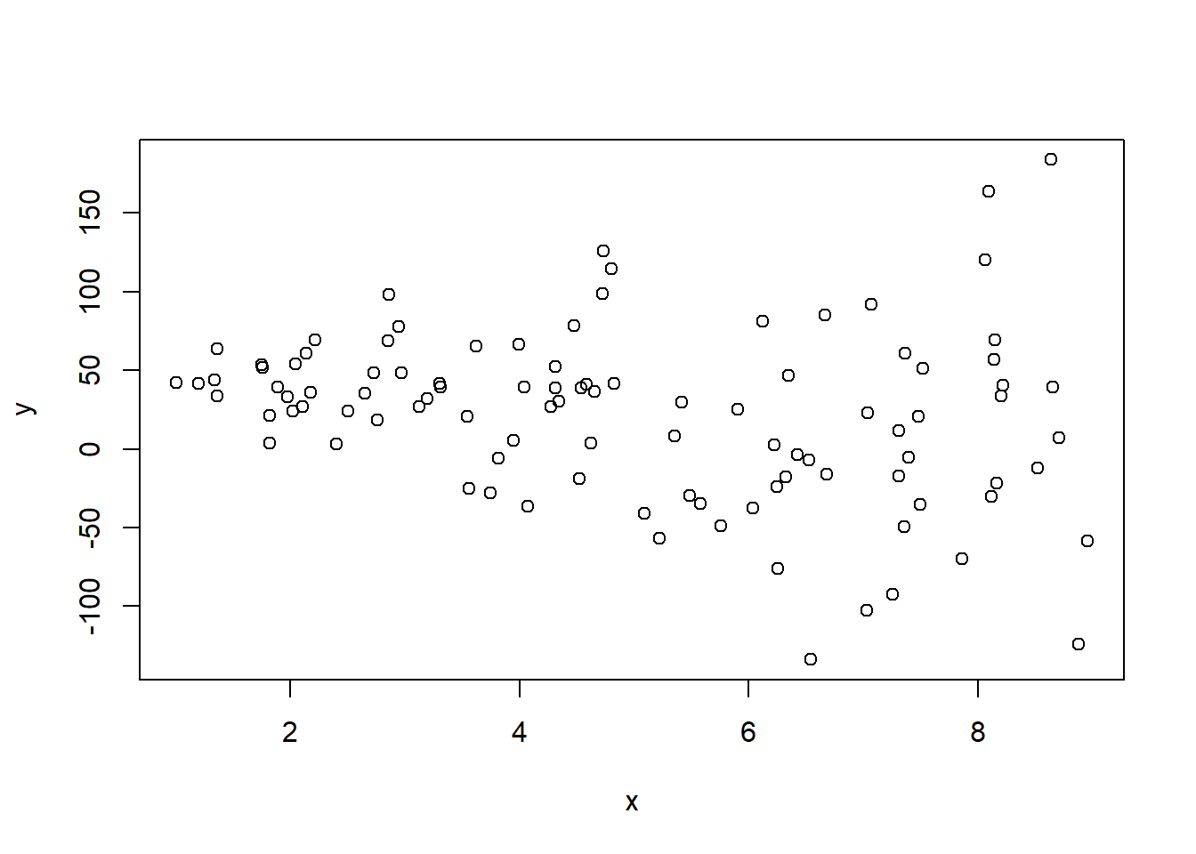
plot(x, y)
- Now let us estimate by OLS and WLS the following empirical model: $$ y = \beta_0 + \beta_1 x + \varepsilon $$
# Estimation
reg.ols = lm(y ~ x) # OLS estimation
reg.wls = lm(y ~ x, weights=1/(10*x)^2) # WLS estimation
stargazer::stargazer(reg.ols, reg.wls, digits=2, type="text", omit.stat="f")
##
## ==========================================================
##                                   Dependent variable:
##                               ----------------------------
##                                            y
##                                    (1)            (2)
## ----------------------------------------------------------
## x                                -5.51**       -5.92***
##                                   (2.35)        (1.77)
##
## Constant                         49.27***      51.43***
##                                  (12.87)        (5.50)
##
## ----------------------------------------------------------
## Observations                       100            100
## R2                                 0.05          0.10
## Adjusted R2                        0.04          0.09
## Residual Std. Error (df = 98)     53.30          0.97
## ==========================================================
## Note:                          *p<0.1; **p<0.05; ***p<0.01
- WLS is more efficient here, producing smaller standard errors because we already know that the error variance is proportional to x.
- In practice, it is difficult to know or justify the exact form of heteroskedasticity because we do not observe the true variance model.
- Below we estimate the model with incorrect weights, $ Var(\tilde{\varepsilon}_i | x_i) = \sigma^2 \left(\frac{1}{10 x_i}\right)^2$. Note that this even affects the coefficient estimates, in addition to worsening the standard errors:
# Estimation
reg.wls2 = lm(y ~ x, weights=x^2) # WLS estimation
stargazer::stargazer(reg.ols, reg.wls, reg.wls2, digits=2, type="text", omit.stat="f")
##
## ===========================================================
##                                    Dependent variable:
##                               -----------------------------
##                                             y
##                                  (1)        (2)      (3)
## -----------------------------------------------------------
## x                              -5.51**   -5.92***   -2.60
##                                 (2.35)    (1.77)    (3.88)
##
## Constant                       49.27***  51.43***   30.54
##                                (12.87)    (5.50)   (26.90)
##
## -----------------------------------------------------------
## Observations                     100        100      100
## R2                               0.05      0.10     0.005
## Adjusted R2                      0.04      0.09     -0.01
## Residual Std. Error (df = 98)   53.30      0.97     368.51
## ===========================================================
## Note:                           *p<0.1; **p<0.05; ***p<0.01
Analytical Estimation
a) Create the vectors/matrices and define N and K
# Create the y vector
y = as.matrix(y) # convert the data-frame column to a matrix

# Create the covariate matrix X with a leading column of ones
X = as.matrix( cbind(1, x) ) # bind the column of ones to x

# Store the values of N and K
N = nrow(X)
K = ncol(X) - 1
b) Weight matrix $\boldsymbol{W}$
- This is the matrix whose main diagonal is filled with the weights, $w_i = 1/x^2_i$
W = diag(1/x^2)
round(W[1:10,1:10], 2)
##       [,1] [,2] [,3] [,4] [,5] [,6] [,7] [,8] [,9] [,10]
##  [1,] 0.09 0.00 0.00 0.00 0.00 0.00 0.00 0.00 0.00  0.00
##  [2,] 0.00 0.02 0.00 0.00 0.00 0.00 0.00 0.00 0.00  0.00
##  [3,] 0.00 0.00 0.05 0.00 0.00 0.00 0.00 0.00 0.00  0.00
##  [4,] 0.00 0.00 0.00 0.02 0.00 0.00 0.00 0.00 0.00  0.00
##  [5,] 0.00 0.00 0.00 0.00 0.01 0.00 0.00 0.00 0.00  0.00
##  [6,] 0.00 0.00 0.00 0.00 0.00 0.54 0.00 0.00 0.00  0.00
##  [7,] 0.00 0.00 0.00 0.00 0.00 0.00 0.04 0.00 0.00  0.00
##  [8,] 0.00 0.00 0.00 0.00 0.00 0.00 0.00 0.02 0.00  0.00
##  [9,] 0.00 0.00 0.00 0.00 0.00 0.00 0.00 0.00 0.03  0.00
## [10,] 0.00 0.00 0.00 0.00 0.00 0.00 0.00 0.00 0.00  0.05
c) WLS estimates $\hat{\boldsymbol{\beta}}_{\scriptscriptstyle{WLS}}$
$$ \hat{\boldsymbol{\beta}}_{\scriptscriptstyle{WLS}} = (\boldsymbol{X}' \boldsymbol{W} \boldsymbol{X})^{-1} \boldsymbol{X}' \boldsymbol{W} \boldsymbol{y} $$bhat_wls = solve( t(X) %*% W %*% X ) %*% t(X) %*% W %*% y
bhat_wls
##        [,1]
##   51.433290
## x -5.923353
d) Fitted values $\hat{\boldsymbol{y}}_{\scriptscriptstyle{WLS}}$
yhat_wls = X %*% bhat_wls
head(yhat_wls)
##            [,1]
## [1,] 31.8825514
## [2,]  8.1546597
## [3,] 26.1298192
## [4,]  3.6665460
## [5,]  0.9441786
## [6,] 43.3511590
e) Residuals $\hat{\boldsymbol{\varepsilon}}_{\scriptscriptstyle{WLS}}$
ehat_wls = y - yhat_wls
head(ehat_wls)
##             [,1]
## [1,]   9.9754298
## [2,]   3.2273830
## [3,]   0.6797571
## [4,] 116.3787515
## [5,] -12.8069979
## [6,]  20.5180944
f) Error variance estimate $\hat{\sigma}^2_{\scriptscriptstyle{WLS}}$ $$\hat{\sigma}^2 = \frac{\hat{\boldsymbol{\varepsilon}}' \boldsymbol{W} \hat{\boldsymbol{\varepsilon}}}{N - K - 1} $$
sig2hat_wls = as.numeric( t(ehat_wls) %*% W %*% ehat_wls / (N-K-1) )
sig2hat_wls
## [1] 93.95364
h) Variance-Covariance Matrix of the Estimator
$$ \widehat{\text{Var}}(\hat{\boldsymbol{\beta}}_{\scriptscriptstyle{WLS}}) = \hat{\sigma}^2 (\boldsymbol{X}' \boldsymbol{W} \boldsymbol{X})^{-1} $$Vbhat_wls = sig2hat_wls * solve( t(X) %*% W %*% X )
round(Vbhat_wls, 3)
##               x
##   30.248 -8.144
## x -8.144  3.132
i) Standard Errors, t Statistics, and p-values
se_wls = sqrt( diag(Vbhat_wls) )
t_wls = bhat_wls / se_wls
p_wls = 2 * pt(-abs(t_wls), N-K-1)

# Results
data.frame(bhat_wls, se_wls, t_wls, p_wls) # WLS results
##    bhat_wls   se_wls     t_wls        p_wls
##   51.433290 5.499861  9.351743 3.090884e-15
## x -5.923353 1.769796 -3.346913 1.159943e-03
summary(reg.wls)$coef # WLS results via lm()
##              Estimate Std. Error   t value     Pr(>|t|)
## (Intercept) 51.433290   5.499861  9.351743 3.090884e-15
## x           -5.923353   1.769796 -3.346913 1.159943e-03
Transforming and Estimating by OLS
- We can now transform the variables and solve by OLS, pre-multiplying $\boldsymbol{X}$ and $\boldsymbol{y}$ by $ \boldsymbol{W}^{0.5}$, and defining:
b’) Weight matrix $\boldsymbol{W}^{0.5}$
- This is the matrix whose main diagonal is filled with the square roots of the weights.
W_0.5 = diag(1/(10*x))
round(W_0.5[1:10,1:10], 2)
##       [,1] [,2] [,3] [,4] [,5] [,6] [,7] [,8] [,9] [,10]
##  [1,] 0.03 0.00 0.00 0.00 0.00 0.00 0.00 0.00 0.00  0.00
##  [2,] 0.00 0.01 0.00 0.00 0.00 0.00 0.00 0.00 0.00  0.00
##  [3,] 0.00 0.00 0.02 0.00 0.00 0.00 0.00 0.00 0.00  0.00
##  [4,] 0.00 0.00 0.00 0.01 0.00 0.00 0.00 0.00 0.00  0.00
##  [5,] 0.00 0.00 0.00 0.00 0.01 0.00 0.00 0.00 0.00  0.00
##  [6,] 0.00 0.00 0.00 0.00 0.00 0.07 0.00 0.00 0.00  0.00
##  [7,] 0.00 0.00 0.00 0.00 0.00 0.00 0.02 0.00 0.00  0.00
##  [8,] 0.00 0.00 0.00 0.00 0.00 0.00 0.00 0.01 0.00  0.00
##  [9,] 0.00 0.00 0.00 0.00 0.00 0.00 0.00 0.00 0.02  0.00
## [10,] 0.00 0.00 0.00 0.00 0.00 0.00 0.00 0.00 0.00  0.02
b’’) Transformed variables $\tilde{\boldsymbol{y}}$ and $\tilde{\boldsymbol{X}}$
ytil = W_0.5 %*% y
Xtil = W_0.5 %*% X
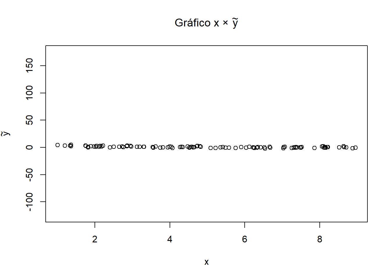
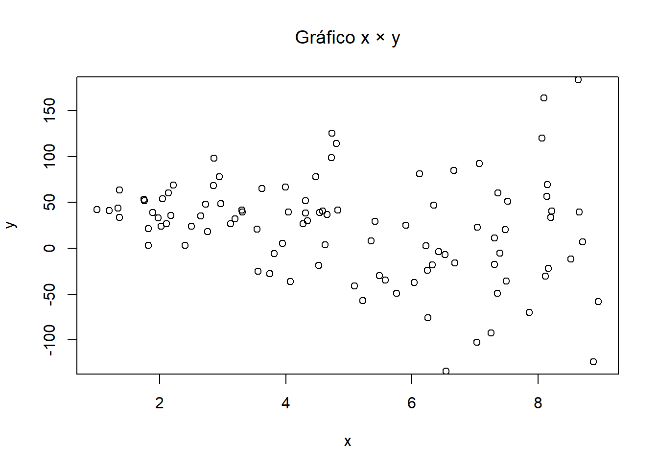
# Plots
plot(x, ytil, ylim=c(-125,175),
main=expression(paste("Plot ", x ," \u00D7 ", tilde(y))),
xlab=expression(x), ylab=expression(tilde(y))) # plot x_tilde and y_tilde
plot(x, y, ylim=c(-125,175),
     main=expression(paste("Plot ", x ," \u00D7 ", y)),
     xlab=expression(x), ylab=expression(y)) # plot x and y
c’) OLS estimates $\tilde{\hat{\boldsymbol{\beta}}}_{\scriptscriptstyle{OLS}}$
$$ \tilde{\hat{\boldsymbol{\beta}}}_{\scriptscriptstyle{OLS}} = (\tilde{\boldsymbol{X}}' \tilde{\boldsymbol{X}})^{-1} \tilde{\boldsymbol{X}}' \tilde{\boldsymbol{y}} $$bhat_ols = solve( t(Xtil) %*% Xtil ) %*% t(Xtil) %*% ytil
bhat_ols
##        [,1]
##   51.433290
## x -5.923353
d’) Fitted values $\tilde{\hat{\boldsymbol{y}}}_{\scriptscriptstyle{OLS}}$
yhat_ols = Xtil %*% bhat_ols
head(yhat_ols)
##            [,1]
## [1,] 0.96595639
## [2,] 0.11160919
## [3,] 0.61167951
## [4,] 0.04546730
## [5,] 0.01107705
## [6,] 3.17718463
e’) Residuals $\tilde{\hat{\boldsymbol{\varepsilon}}}_{\scriptscriptstyle{OLS}}$
ehat_ols = ytil - yhat_ols
head(ehat_ols)
##             [,1]
## [1,]  0.30222895
## [2,]  0.04417175
## [3,]  0.01591261
## [4,]  1.44316397
## [5,] -0.15025095
## [6,]  1.50376081
f’) Error variance estimate $\tilde{\hat{\sigma}}^2_{\scriptscriptstyle{OLS}}$ $$\tilde{\hat{\sigma}}^2 = \frac{\tilde{\hat{\boldsymbol{\varepsilon}}}' \tilde{\hat{\boldsymbol{\varepsilon}}}}{N - K - 1} $$
sig2hat_ols = as.numeric( t(ehat_ols) %*% ehat_ols / (N-K-1) )
sig2hat_ols
## [1] 0.9395364
h’) Variance-Covariance Matrix of the Estimator
$$ \widehat{\text{Var}}(\hat{\boldsymbol{\beta}}_{\scriptscriptstyle{OLS}}) = \tilde{\hat{\sigma}}^2(\tilde{\boldsymbol{X}}' \tilde{\boldsymbol{X}})^{-1} $$Vbhat_ols = sig2hat_ols * solve( t(Xtil) %*% Xtil )
round(Vbhat_ols, 3)
##               x
##   30.248 -8.144
## x -8.144  3.132
i’) Standard Errors, t Statistics, and p-values
se_ols = sqrt( diag(Vbhat_ols) )
t_ols = bhat_ols / se_ols
p_ols = 2 * pt(-abs(t_ols), N-K-1)

# Results
data.frame(bhat_ols, se_ols, t_ols, p_ols) # transformed OLS results
##    bhat_ols   se_ols     t_ols        p_ols
##   51.433290 5.499861  9.351743 3.090884e-15
## x -5.923353 1.769796 -3.346913 1.159943e-03
summary(reg.wls)$coef # WLS results via lm()
##              Estimate Std. Error   t value     Pr(>|t|)
## (Intercept) 51.433290   5.499861  9.351743 3.090884e-15
## x           -5.923353   1.769796 -3.346913 1.159943e-03
FGLS Estimator
In practice, it is difficult to know the error variance-covariance matrix a priori.
A reasonable approach is to assume that $\boldsymbol{\Sigma}$ is a function of unknown parameters from a linear model, collected in $\boldsymbol{\gamma}$.
We can then estimate $\hat{\boldsymbol{\gamma}}$ from OLS residuals and use it to construct $\boldsymbol{\Sigma}(\hat{\boldsymbol{\gamma}})$.
This procedure is known as Feasible Generalized Least Squares (FGLS), because its calculation is feasible even when GLS itself is not.
Note that if $\boldsymbol{\Sigma}(\hat{\boldsymbol{\gamma}})$ is a poor approximation to $\boldsymbol{\Sigma}$, then the resulting FGLS estimates and inference may perform poorly.
We want to estimate the model $$y_i = \beta_0 + \beta_1 x_{i1} + ... + \beta_K x_{iK} + \varepsilon_i = \boldsymbol{x}'_i \boldsymbol{\beta} + \varepsilon_i, \tag{1} $$ while the individual error variance is typically assumed to be given by: $$Var(\varepsilon_i | \boldsymbol{x}'_i) = \sigma^2 \exp(\boldsymbol{x}'_i \boldsymbol{\gamma}). $$
The function $\exp(\boldsymbol{x}'_i \boldsymbol{\gamma})$ is an example of a skedastic function, ensuring that the fitted value is never negative after estimating $\hat{\boldsymbol{\gamma}}$ and thus keeping the variance positive for every individual.
To estimate $\boldsymbol{\gamma}$, we need consistent estimates of $\hat{\boldsymbol{\varepsilon}}$. The usual starting point is to compute $\hat{\boldsymbol{\varepsilon}}_{\scriptscriptstyle{OLS}}$.
Next, we run the auxiliary linear regression $$ \log{\hat{\varepsilon}}^2_i = \boldsymbol{x}'_i \boldsymbol{\gamma} + u_i, \tag{2} $$
From that estimation, we use the fitted values to compute $$h(\boldsymbol{x}'_i) = \exp(\boldsymbol{x}'_i \boldsymbol{\gamma})$$ which is the inverse of the weight $$w_i = \frac{1}{h(\boldsymbol{x}'_i)} = \frac{1}{\exp(\boldsymbol{x}'_i \boldsymbol{\gamma})}$$
With the estimated $\boldsymbol{W}$, we can compute $\hat{\boldsymbol{\beta}}_{\scriptscriptstyle{FGLS}}$ and $V(\hat{\boldsymbol{\beta}}_{\scriptscriptstyle{FGLS}})$, following the same steps as for WLS.
We can then use the estimated $\hat{\boldsymbol{\beta}}_{\scriptscriptstyle{FGLS}}$ to estimate a new $\boldsymbol{\gamma}$ and a new $\hat{\boldsymbol{\beta}}_{\scriptscriptstyle{FGLS}}$. This can be iterated until convergence (if it occurs) or for a fixed number of iterations.
Estimation via lm()
data(smoke, package="wooldridge")

# OLS estimation
reg.ols = lm(cigs ~ lincome + lcigpric + educ + age + agesq + restaurn,
             data=smoke)
round(summary(reg.ols)$coef, 4)
##             Estimate Std. Error t value Pr(>|t|)
## (Intercept)  -3.6398    24.0787 -0.1512   0.8799
## lincome       0.8803     0.7278  1.2095   0.2268
## lcigpric     -0.7509     5.7733 -0.1301   0.8966
## educ         -0.5015     0.1671 -3.0016   0.0028
## age           0.7707     0.1601  4.8132   0.0000
## agesq        -0.0090     0.0017 -5.1765   0.0000
## restaurn     -2.8251     1.1118 -2.5410   0.0112
# Obtain the weights w_i = 1/h(z_i) = 1/exp(Xg)
logu2 = log(resid(reg.ols)^2)
reg.var = lm(logu2 ~ lincome + lcigpric + educ + age + agesq + restaurn,
             data=smoke)
w = 1/exp(fitted(reg.var))

# FGLS estimation
reg.fgls = lm(cigs ~ lincome + lcigpric + educ + age + agesq + restaurn,
              weight=w, data=smoke)
round(summary(reg.fgls)$coef, 4)
##             Estimate Std. Error t value Pr(>|t|)
## (Intercept)   5.6355    17.8031  0.3165   0.7517
## lincome       1.2952     0.4370  2.9639   0.0031
## lcigpric     -2.9403     4.4601 -0.6592   0.5099
## educ         -0.4634     0.1202 -3.8570   0.0001
## age           0.4819     0.0968  4.9784   0.0000
## agesq        -0.0056     0.0009 -5.9897   0.0000
## restaurn     -3.4611     0.7955 -4.3508   0.0000
Analytical Estimation
- This is similar to WLS; only the beginning changes: a) Create the vectors/matrices and define N and K
# Create the y vector
y = as.matrix(smoke[,"cigs"]) # convert the data-frame column to a matrix

# Create the covariate matrix X with a leading column of ones
X = as.matrix( cbind(1, smoke[,c("lincome", "lcigpric", "educ", "age", "agesq",
                                 "restaurn")]) ) # bind the column of ones to x

# Store the values of N and K
N = nrow(X)
K = ncol(X) - 1
b1) OLS estimation to obtain $\hat{\boldsymbol{\varepsilon}}_{\scriptscriptstyle{OLS}}$
bhat_ols = solve(t(X) %*% X) %*% t(X) %*% y
yhat = X %*% bhat_ols
ehat = y - yhat
b2) Regress the log squared residuals and estimate $\hat{\boldsymbol{\gamma}}$ $$ \log{\hat{\boldsymbol{\varepsilon}}}^2 = \boldsymbol{X} \boldsymbol{\gamma} + \boldsymbol{u} $$
ghat = solve( t(X) %*% X ) %*% t(X) %*% log(ehat^2)
b3) Weight matrix $\boldsymbol{W}$ $$\boldsymbol{W} = diag\left(\frac{1}{\exp(\boldsymbol{X} \hat{\boldsymbol{\gamma}})}\right) = \begin{bmatrix} \frac{1}{\exp(\boldsymbol{x}'_1\hat{\boldsymbol{\gamma}})} & 0 & \cdots & 0 \\ 0 & \frac{1}{\exp(\boldsymbol{x}'_2\hat{\boldsymbol{\gamma}})} & \cdots & 0 \\ \vdots & \vdots & \ddots & \vdots \\ 0 & 0 & \cdots & \frac{1}{\exp(\boldsymbol{x}'_N\hat{\boldsymbol{\gamma}})} \end{bmatrix}$$
W = diag(as.numeric(1 / exp(X %*% ghat)))
round(W[1:7,1:7], 3)
##       [,1]  [,2]  [,3] [,4]  [,5]  [,6]  [,7]
## [1,] 0.008 0.000 0.000 0.00 0.000 0.000 0.000
## [2,] 0.000 0.007 0.000 0.00 0.000 0.000 0.000
## [3,] 0.000 0.000 0.009 0.00 0.000 0.000 0.000
## [4,] 0.000 0.000 0.000 0.01 0.000 0.000 0.000
## [5,] 0.000 0.000 0.000 0.00 0.024 0.000 0.000
## [6,] 0.000 0.000 0.000 0.00 0.000 0.444 0.000
## [7,] 0.000 0.000 0.000 0.00 0.000 0.000 0.007
- The remaining steps are the same as in WLS:
c) FGLS estimates $\hat{\boldsymbol{\beta}}_{\scriptscriptstyle{FGLS}}$ $$ \hat{\boldsymbol{\beta}}_{\scriptscriptstyle{FGLS}} = (\boldsymbol{X}' \boldsymbol{W} \boldsymbol{X})^{-1} \boldsymbol{X}' \boldsymbol{W} \boldsymbol{y} $$
bhat_fgls = solve( t(X) %*% W %*% X ) %*% t(X) %*% W %*% y
bhat_fgls
##                 [,1]
## 1         5.63546183
## lincome   1.29523990
## lcigpric -2.94031229
## educ     -0.46344637
## age       0.48194788
## agesq    -0.00562721
## restaurn -3.46106414
d) Fitted values $\hat{\boldsymbol{y}}_{\scriptscriptstyle{FGLS}}$
yhat_fgls = X %*% bhat_fgls
head(yhat_fgls)
##        [,1]
## 1  9.246793
## 2  9.914233
## 3 10.527827
## 4  9.667243
## 5  8.440092
## 6  2.048962
e) Residuals $\hat{\boldsymbol{\varepsilon}}_{\scriptscriptstyle{FGLS}}$
ehat_fgls = y - yhat_fgls
head(ehat_fgls)
##        [,1]
## 1 -9.246793
## 2 -9.914233
## 3 -7.527827
## 4 -9.667243
## 5 -8.440092
## 6 -2.048962
f) Error variance estimate $\hat{\sigma}^2_{\scriptscriptstyle{FGLS}}$ $$\hat{\sigma}^2 = \frac{\hat{\boldsymbol{\varepsilon}}' \boldsymbol{W} \hat{\boldsymbol{\varepsilon}}}{N - K - 1} $$
sig2hat_fgls = as.numeric( t(ehat_fgls) %*% W %*% ehat_fgls / (N-K-1) )
sig2hat_fgls
## [1] 2.492289
h) Variance-Covariance Matrix of the Estimator
$$ \widehat{\text{Var}}(\hat{\boldsymbol{\beta}}_{\scriptscriptstyle{FGLS}}) = (\boldsymbol{X}' \boldsymbol{W} \boldsymbol{X})^{-1} $$Vbhat_fgls = sig2hat_fgls * solve( t(X) %*% W %*% X )
round(Vbhat_fgls, 3)
##                1 lincome lcigpric   educ    age  agesq restaurn
## 1        316.952   0.444  -77.432  0.196 -0.389  0.004    2.323
## lincome    0.444   0.191   -0.463 -0.016 -0.007  0.000    0.008
## lcigpric -77.432  -0.463   19.893 -0.050  0.071 -0.001   -0.620
## educ       0.196  -0.016   -0.050  0.014 -0.001  0.000    0.002
## age       -0.389  -0.007    0.071 -0.001  0.009  0.000   -0.009
## agesq      0.004   0.000   -0.001  0.000  0.000  0.000    0.000
## restaurn   2.323   0.008   -0.620  0.002 -0.009  0.000    0.633
i) Standard Errors, t Statistics, and p-values
se_fgls = sqrt( diag(Vbhat_fgls) )
t_fgls = bhat_fgls / se_fgls
p_fgls = 2 * pt(-abs(t_fgls), N-K-1)

# Results
round(data.frame(bhat_fgls, se_fgls, t_fgls, p_fgls), 4) # FGLS results
##          bhat_fgls se_fgls  t_fgls p_fgls
## 1           5.6355 17.8031  0.3165 0.7517
## lincome     1.2952  0.4370  2.9639 0.0031
## lcigpric   -2.9403  4.4601 -0.6592 0.5099
## educ       -0.4634  0.1202 -3.8570 0.0001
## age         0.4819  0.0968  4.9784 0.0000
## agesq      -0.0056  0.0009 -5.9897 0.0000
## restaurn   -3.4611  0.7955 -4.3508 0.0000
round(summary(reg.fgls)$coef, 4) # FGLS results via lm()
##             Estimate Std. Error t value Pr(>|t|)
## (Intercept)   5.6355    17.8031  0.3165   0.7517
## lincome       1.2952     0.4370  2.9639   0.0031
## lcigpric     -2.9403     4.4601 -0.6592   0.5099
## educ         -0.4634     0.1202 -3.8570   0.0001
## age           0.4819     0.0968  4.9784   0.0000
## agesq        -0.0056     0.0009 -5.9897   0.0000
## restaurn     -3.4611     0.7955 -4.3508   0.0000