- We now turn to more general hypothesis tests that are not usually reported directly in standard regression output.
Wald Test
Consider:
- $G$: the number of linear restrictions
- $\boldsymbol{\beta}$: a $(K+1) \times 1$ parameter vector
- $\boldsymbol{h}$: a $G \times 1$ vector of constants
- $\boldsymbol{R}$: a $G \times (K+1)$ matrix formed by stacking $G$ row vectors $\boldsymbol{r}'_g$ of dimension $1 \times (K+1)$, for $g=1, 2, ..., G$
- A multivariate model:
Using these matrices and vectors, we can write hypothesis tests in the form: \begin{align} \text{H}_0: &\underset{G\times (K+1)}{\boldsymbol{R}} \underset{(K+1)\times 1}{\boldsymbol{\beta}} = \underset{G \times 1}{\boldsymbol{h}} \\ \text{H}_0: &\left[ \begin{matrix} \boldsymbol{r}'_1 \\ \boldsymbol{r}'_2 \\ \vdots \\ \boldsymbol{r}'_{G} \end{matrix} \right] \boldsymbol{\beta} = \left[ \begin{matrix} h_1 \\ h_2 \\ \vdots \\ h_G \end{matrix} \right] \\ \text{H}_0: &\left\{ \begin{matrix} \boldsymbol{r}'_1 \boldsymbol{\beta} = h_1 \\ \boldsymbol{r}'_2 \boldsymbol{\beta} = h_2 \\ \vdots \\ \boldsymbol{r}'_G \boldsymbol{\beta} = h_G \end{matrix} \right. \end{align}
One Linear Restriction
Consider the model: $$y = \beta_0 + \beta_1 x_1 + \beta_2 x_2 + \varepsilon$$
There are $K=2$ explanatory variables (and therefore 3 parameters).
One linear restriction $\Longrightarrow \ G=1$
In this particular case, we have $$\boldsymbol{R} = \boldsymbol{r}'_1\ \implies\ \text{H}_0:\ \boldsymbol{r}'_1 \boldsymbol{\beta} = h_1 $$
Evaluating the Null Hypothesis with a Single Restriction
With a single restriction, we assume that $$ \boldsymbol{r}'_1 \hat{\boldsymbol{\beta}} \sim N(\boldsymbol{r}'_1 \hat{\boldsymbol{\beta}};\ \boldsymbol{r}'_1 \boldsymbol{V(\hat{\boldsymbol{\beta}}) r_1})$$
The Wald statistic is then computed as follows. With a single restriction, it coincides with the usual t statistic: $$ w = t = \frac{\boldsymbol{r}'_1 \hat{\boldsymbol{\beta}} - h_1}{\sqrt{\boldsymbol{r}'_1 \hat{\sigma}^2 (\boldsymbol{X}'\boldsymbol{X})^{-1} \boldsymbol{r}_1}} = \frac{\boldsymbol{r}'_1 \hat{\boldsymbol{\beta}} - h_1}{\sqrt{\boldsymbol{r}'_1 \boldsymbol{V(\hat{\boldsymbol{\beta}})} \boldsymbol{r}_1}} $$
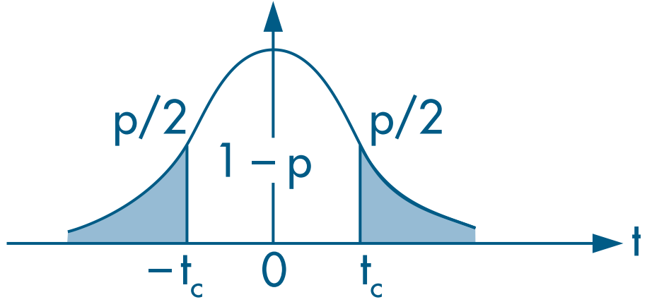
Choose a significance level $\alpha$ and reject the null hypothesis when the t statistic lies outside the relevant confidence interval.
Example 1: H$_0: \ \beta_1 = 4$
- Note that $h_1 = 4$.
- The vector $r'_1$ can be written as
So the null hypothesis is $$\text{H}_0:\ \boldsymbol{r}'_1 \boldsymbol{\beta}\ =\ \left[ \begin{matrix} 0 & 1 & 0 \end{matrix} \right] \left[ \begin{matrix} \beta_0 \\ \beta_1 \\ \beta_2 \end{matrix} \right] = 4\ \iff\ \beta_1 = 4 $$
And the denominator of the t statistic is: \begin{align} &\sqrt{\boldsymbol{r}'_1 \boldsymbol{V(\hat{\boldsymbol{\beta}})} \boldsymbol{r}_1} \\ &= \sqrt{\left[ \begin{matrix} 0 & 1 & 0 \end{matrix} \right] {\small \begin{bmatrix} var(\hat{\beta}_0) & cov(\hat{\beta}_0, \hat{\beta}_1) & cov(\hat{\beta}_0, \hat{\beta}_2) \\ cov(\hat{\beta}_0, \hat{\beta}_1) & var(\hat{\beta}_1) & cov(\hat{\beta}_1, \hat{\beta}_2) \\ cov(\hat{\beta}_0, \hat{\beta}_2) & cov(\hat{\beta}_1, \hat{\beta}_2) & var(\hat{\beta}_2) \\ \end{bmatrix}} \left[ \begin{matrix} 0 \\ 1 \\ 0 \end{matrix} \right]} \\ &= \sqrt{\small{\begin{bmatrix} cov(\hat{\beta}_0, \hat{\beta}_1) & var(\hat{\beta}_1) & cov(\hat{\beta}_1, \hat{\beta}_2) \end{bmatrix}} \left[ \begin{matrix} 0 \\ 1 \\ 0 \end{matrix} \right]} \\ &= \sqrt{var(\hat{\beta}_1)} = se(\hat{\beta}_1) \end{align}
Example 2: H$_0: \ \beta_1 + \beta_2 = 2$
- Note that $h_1 = 2$.
- The vector $r'_1$ can be written as
So the null hypothesis is $$\text{H}_0:\ \boldsymbol{r}'_1 \boldsymbol{\beta}\ =\ \left[ \begin{matrix} 0 & 1 & 1 \end{matrix} \right] \left[ \begin{matrix} \beta_0 \\ \beta_1 \\ \beta_2 \end{matrix} \right] = 2\ \iff\ \beta_1 + \beta_2 = 2 $$
And the denominator of the t statistic is: \begin{align} &\sqrt{\boldsymbol{r}'_1 \boldsymbol{V(\hat{\boldsymbol{\beta}})} \boldsymbol{r}_1} \\ &= \sqrt{\left[ \begin{matrix} 0 & 1 & 1 \end{matrix} \right] {\small \begin{bmatrix} var(\hat{\beta}_0) & cov(\hat{\beta}_0, \hat{\beta}_1) & cov(\hat{\beta}_0, \hat{\beta}_2) \\ cov(\hat{\beta}_0, \hat{\beta}_1) & var(\hat{\beta}_1) & cov(\hat{\beta}_1, \hat{\beta}_2) \\ cov(\hat{\beta}_0, \hat{\beta}_2) & cov(\hat{\beta}_1, \hat{\beta}_2) & var(\hat{\beta}_2) \\ \end{bmatrix}} \left[ \begin{matrix} 0 \\ 1 \\ 1 \end{matrix} \right]} \\ &= \sqrt{\small{\begin{bmatrix} cov(\hat{\beta}_0, \hat{\beta}_1)+cov(\hat{\beta}_0, \hat{\beta}_2) \\ var(\hat{\beta}_1) + cov(\hat{\beta}_1, \hat{\beta}_2) \\ cov(\hat{\beta}_1, \hat{\beta}_2) + var(\hat{\beta}_2) \end{bmatrix}}' \left[ \begin{matrix} 0 \\ 1 \\ 1 \end{matrix} \right]} \\ &= \sqrt{var(\hat{\beta}_1) + var(\hat{\beta}_2) + 2cov(\hat{\beta}_1, \hat{\beta}_2)} = \sqrt{var(\hat{\beta}_1 + \hat{\beta}_2)} \end{align}
Example 3: H$_0: \ \beta_1 = \beta_2$
Note that $$\beta_1 = \beta_2 \iff \beta_1 - \beta_2 = 0 $$
Hence, $h_1 = 0$.
The vector $r'_1$ can be written as
So the null hypothesis is $$\text{H}_0:\ \boldsymbol{r}'_1 \boldsymbol{\beta}\ =\ \left[ \begin{matrix} 0 & 1 & -1 \end{matrix} \right] \left[ \begin{matrix} \beta_0 \\ \beta_1 \\ \beta_2 \end{matrix} \right] = 0\ \iff\ \beta_1 - \beta_2 = 0 $$
And the denominator of the t statistic is: \begin{align} &\sqrt{\boldsymbol{r}'_1 \boldsymbol{V(\hat{\boldsymbol{\beta}})} \boldsymbol{r}_1} \\ &= \sqrt{\left[ \begin{matrix} 0 & 1 & -1 \end{matrix} \right] {\small \begin{bmatrix} var(\hat{\beta}_0) & cov(\hat{\beta}_0, \hat{\beta}_1) & cov(\hat{\beta}_0, \hat{\beta}_2) \\ cov(\hat{\beta}_0, \hat{\beta}_1) & var(\hat{\beta}_1) & cov(\hat{\beta}_1, \hat{\beta}_2) \\ cov(\hat{\beta}_0, \hat{\beta}_2) & cov(\hat{\beta}_1, \hat{\beta}_2) & var(\hat{\beta}_2) \\ \end{bmatrix}} \left[ \begin{matrix} 0 \\ 1 \\ -1 \end{matrix} \right]} \\ &= \sqrt{\small{\begin{bmatrix} cov(\hat{\beta}_0, \hat{\beta}_1)-cov(\hat{\beta}_0, \hat{\beta}_2) \\ var(\hat{\beta}_1) - cov(\hat{\beta}_1, \hat{\beta}_2) \\ cov(\hat{\beta}_1, \hat{\beta}_2) - var(\hat{\beta}_2) \end{bmatrix}}' \left[ \begin{matrix} 0 \\ 1 \\ -1 \end{matrix} \right]} \\ &= \sqrt{var(\hat{\beta}_1) + var(\hat{\beta}_2) - 2cov(\hat{\beta}_1, \hat{\beta}_2)} = \sqrt{var(\hat{\beta}_1 - \hat{\beta}_2)} \end{align}
Implementing It in R
(Continued) Example 7.5: Log Hourly Wage Equation (Wooldridge, 2006)
- Earlier, we estimated the following model:
\begin{align} \log(\text{wage}) = &\beta_0 + \beta_1 \text{female} + \beta_2 \text{married} + \delta_2 \text{female*married} + \beta_3 \text{educ} +\\ &\beta_4 \text{exper} + \beta_5 \text{exper}^2 + \beta_6 \text{tenure} + \beta_7 \text{tenure}^2 + \varepsilon \end{align} where:
wage: average hourly wagefemale: dummy equal to (1) for women and (0) for menmarried: dummy equal to (1) for married individuals and (0) otherwisefemale*married: interaction term between thefemaleandmarrieddummieseduc: years of educationexper: years of experience (expersq= years squared)tenure: years with the current employer (tenursq= years squared)
# Loading the required dataset
data(wage1, package="wooldridge")

# Estimating the model
res_7.14 = lm(lwage ~ female*married + educ + exper + expersq + tenure + tenursq, data=wage1)
round( summary(res_7.14)$coef, 4 )
##                Estimate Std. Error t value Pr(>|t|)
## (Intercept)      0.3214     0.1000  3.2135   0.0014
## female          -0.1104     0.0557 -1.9797   0.0483
## married          0.2127     0.0554  3.8419   0.0001
## educ             0.0789     0.0067 11.7873   0.0000
## exper            0.0268     0.0052  5.1118   0.0000
## expersq         -0.0005     0.0001 -4.8471   0.0000
## tenure           0.0291     0.0068  4.3016   0.0000
## tenursq         -0.0005     0.0002 -2.3056   0.0215
## female:married  -0.3006     0.0718 -4.1885   0.0000
- We can see that the effect of marriage for women differs from the effect for men because the coefficient on
female:married( $\delta_2$) is statistically significant. - However, to determine whether the effect of marriage for women is itself significant, we need to test whether H$_0 :\ \beta_2 + \delta_2 = 0$.
- Because there is only one restriction, we can evaluate this hypothesis with a t test:
# Extracting objects from the regression
bhat = matrix(coef(res_7.14), ncol=1) # coefficients as a column vector
Vbhat = vcov(res_7.14) # variance-covariance matrix of the estimator
N = nrow(wage1) # number of observations
K = length(bhat) - 1 # number of covariates
ehat = residuals(res_7.14) # regression residuals

# Building the row vector for the restriction
r1prime = matrix(c(0, 0, 1, 0, 0, 0, 0, 0, 1), nrow=1) # restriction vector
h1 = 0 # constant in H0
G = 1 # number of restrictions

# Computing the t statistic
t = (r1prime %*% bhat - h1) / sqrt(r1prime %*% Vbhat %*% t(r1prime))
abs(t)
##          [,1]
## [1,] 1.679475
# Computing the p-value
p = 2 * pt(-abs(t), N-K-1)
p
##            [,1]
## [1,] 0.09366368
Since $|t| < 2$ (an approximate critical value for a 5% significance level), we do not reject the null hypothesis and conclude that the effect of marriage on women’s wages ( $\beta_2 + \delta_2$) is not statistically significant.
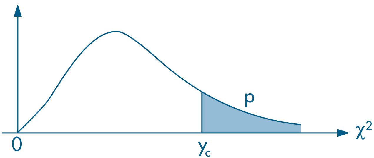
We can also assess the same restriction with a Wald test, evaluating the statistic against a $\chi^2$ distribution with 1 degree of freedom (because there is only $G=1$ restriction).
Recall that the chi-squared test is right-tailed.
# Computing the Wald statistic
aux = r1prime %*% bhat - h1 # R \beta - h
w = t(aux) %*% solve( r1prime %*% Vbhat %*% t(r1prime)) %*% aux
w
##          [,1]
## [1,] 2.820636
# Computing the p-value for w
p = 1 - pchisq(w, df=G)
p
##            [,1]
## [1,] 0.09305951
Multiple Linear Restrictions
Evaluating the Null Hypothesis with Multiple Restrictions
With G restrictions, we assume that $$ \boldsymbol{R} \hat{\boldsymbol{\beta}} \sim N(\boldsymbol{R} \hat{\boldsymbol{\beta}};\ \sigma^2 \boldsymbol{R} \boldsymbol{V(\hat{\boldsymbol{\beta}}) R'})$$
The Wald statistic is then $$ w = \left[ \boldsymbol{R}\hat{\boldsymbol{\beta}} - \boldsymbol{h} \right]' \left[ \boldsymbol{R V(\hat{\beta}) R}' \right]^{-1} \left[ \boldsymbol{R}\hat{\boldsymbol{\beta}} - \boldsymbol{h} \right]\ \sim\ \chi^2_{(G)} $$
Choose a significance level $\alpha$ and reject the null hypothesis when the statistic $w$ falls outside the acceptance region (from zero to the critical value).
Example 4: H$_0: \ \beta_1 = 0\ \text{ e }\ \beta_1 + \beta_2 = 2$
- Note that $h_1 = 0 \text{ and } h_2 = 2$.
- The vectors $r'_1 \text{ and } r'_2$ can be written as
Therefore, $\boldsymbol{R}$ is $$ \boldsymbol{R} = \left[ \begin{matrix} \boldsymbol{r}'_1 \\ \boldsymbol{r}'_2 \end{matrix} \right] = \left[ \begin{matrix} 0 & 1 & 0 \\ 0 & 1 & 1 \end{matrix} \right] $$
So the null hypothesis is $$\text{H}_0:\ \boldsymbol{R} \boldsymbol{\beta} = \left[ \begin{matrix} 0 & 1 & 0 \\ 0 & 1 & 1 \end{matrix} \right] \left[ \begin{matrix} \beta_0 \\ \beta_1 \\ \beta_2 \end{matrix} \right] = \left[ \begin{matrix} h_1 \\ h_2 \end{matrix} \right]\ \iff\ \text{H}_0:\ \left\{ \begin{matrix} \beta_1 &= 0 \\ \beta_1 + \beta_2 &= 2 \end{matrix} \right. $$
Implementing It in R
- As an example, we use the
mlb1dataset from thewooldridgepackage, which contains baseball-player statistics (Wooldridge, 2006, Section 4.5). - We want to estimate the model:
\begin{align} \log(\text{salary}) = &\beta_0 + \beta_1. \text{years} + \beta_2. \text{gameyr} + \beta_3. \text{bavg} + \\
&\beta_4 .\text{hrunsyr} + \beta_5. \text{rbisyr} + \varepsilon \end{align}
where:
log(salary): log salary in 1993years: years spent in Major League Baseballgamesyr: average number of games per yearbavg: career batting averagehrunsyr: average number of home runs per yearrbisyr: average number of runs batted in per year
data(mlb1, package="wooldridge")

# Estimating the full (unrestricted) model
resMLB = lm(log(salary) ~ years + gamesyr + bavg + hrunsyr + rbisyr, data=mlb1)
round(summary(resMLB)$coef, 5) # estimated coefficients
##             Estimate Std. Error  t value Pr(>|t|)
## (Intercept) 11.19242    0.28882 38.75184  0.00000
## years        0.06886    0.01211  5.68430  0.00000
## gamesyr      0.01255    0.00265  4.74244  0.00000
## bavg         0.00098    0.00110  0.88681  0.37579
## hrunsyr      0.01443    0.01606  0.89864  0.36947
## rbisyr       0.01077    0.00717  1.50046  0.13440
Individually, the variables
bavg,hrunsyr, andrbisyrare not statistically significant.We want to test whether they are jointly significant, that is, $$ \text{H}_0:\ \left\{ \begin{matrix} \beta_3 = 0 \\ \beta_4 = 0 \\ \beta_5 = 0\end{matrix} \right. $$
Thus, we have $$ \boldsymbol{R} = \left[ \begin{matrix} \boldsymbol{r}'_1 \\ \boldsymbol{r}'_2 \\ \boldsymbol{r}'_3 \end{matrix} \right] = \left[ \begin{matrix} 0 & 0 & 0 & 1 & 0 & 0 \\ 0 & 0 & 0 & 0 & 1 & 0 \\ 0 & 0 & 0 & 0 & 0 & 1 \end{matrix} \right] $$
Using Wald.test()
# Extracting the variance-covariance matrix of the estimator
Vbhat = vcov(resMLB)
round(Vbhat, 5)
##             (Intercept)    years  gamesyr     bavg  hrunsyr   rbisyr
## (Intercept)     0.08342  0.00001 -0.00027 -0.00029 -0.00148  0.00082
## years           0.00001  0.00015 -0.00001  0.00000 -0.00002  0.00001
## gamesyr        -0.00027 -0.00001  0.00001  0.00000  0.00002 -0.00002
## bavg           -0.00029  0.00000  0.00000  0.00000  0.00000  0.00000
## hrunsyr        -0.00148 -0.00002  0.00002  0.00000  0.00026 -0.00010
## rbisyr          0.00082  0.00001 -0.00002  0.00000 -0.00010  0.00005
# Computing the Wald statistic
# install.packages("aod") # installing the required package
aod::wald.test(Sigma = Vbhat, # variance-covariance matrix
               b = coef(resMLB), # estimated coefficients
               Terms = 4:6, # positions of the parameters to be tested
               H0 = c(0, 0, 0) # vector h (all equal to zero)
               )
## Wald test:
## ----------
##
## Chi-squared test:
## X2 = 28.7, df = 3, P(> X2) = 2.7e-06
- We reject the null hypothesis and therefore conclude that the parameters $\beta_3, \beta_4 \text{ and } \beta_5$ are jointly significant.
Computing It By Hand
- Estimating the model
# Creating the log_salary variable
mlb1$log_salary = log(mlb1$salary)
name_y = "log_salary"
names_X = c("years", "gamesyr", "bavg", "hrunsyr", "rbisyr")

# Creating the y vector
y = as.matrix(mlb1[,name_y]) # converting a data-frame column to a matrix

# Creating the covariate matrix X with a first column of 1s
X = as.matrix( cbind( const=1, mlb1[,names_X] ) ) # binding a column of 1s to the covariates

# Extracting N and K
N = nrow(mlb1)
K = ncol(X) - 1

# Estimating the model
bhat = solve( t(X) %*% X ) %*% t(X) %*% y
round(bhat, 5)
##             [,1]
## const   11.19242
## years    0.06886
## gamesyr  0.01255
## bavg     0.00098
## hrunsyr  0.01443
## rbisyr   0.01077
# Computing residuals
ehat = y - X %*% bhat

# Variance of the error term
sig2hat = as.numeric( t(ehat) %*% ehat / (N-K-1) )

# Variance-covariance matrix of the estimator
Vbhat = sig2hat * solve( t(X) %*% X )
round(Vbhat, 5)
##            const    years  gamesyr     bavg  hrunsyr   rbisyr
## const    0.08342  0.00001 -0.00027 -0.00029 -0.00148  0.00082
## years    0.00001  0.00015 -0.00001  0.00000 -0.00002  0.00001
## gamesyr -0.00027 -0.00001  0.00001  0.00000  0.00002 -0.00002
## bavg    -0.00029  0.00000  0.00000  0.00000  0.00000  0.00000
## hrunsyr -0.00148 -0.00002  0.00002  0.00000  0.00026 -0.00010
## rbisyr   0.00082  0.00001 -0.00002  0.00000 -0.00010  0.00005
- Next, we build the restriction matrix.
# Number of restrictions
G = 3

# Restriction matrix
R = matrix(c(0, 0, 0, 1, 0, 0,
             0, 0, 0, 0, 1, 0,
             0, 0, 0, 0, 0, 1),
           nrow=G, byrow=TRUE)
R
##      [,1] [,2] [,3] [,4] [,5] [,6]
## [1,]    0    0    0    1    0    0
## [2,]    0    0    0    0    1    0
## [3,]    0    0    0    0    0    1
# Vector of constants h
h = matrix(c(0, 0, 0),
           nrow=3, ncol=1)
h
##      [,1]
## [1,]    0
## [2,]    0
## [3,]    0
- Remember that, by default,
matrix()fills a matrix by column. - Here, however, it is more intuitive to fill the restriction matrix by row, since each row corresponds to one restriction. That is why we used
byrow=TRUE. - The Wald statistic is therefore $$ w(\hat{\boldsymbol{\beta}}) = \left[ \boldsymbol{R}\hat{\boldsymbol{\beta}} - \boldsymbol{h} \right]' \left[ \boldsymbol{R V_{\hat{\beta}} R}' \right]^{-1} \left[ \boldsymbol{R}\hat{\boldsymbol{\beta}} - \boldsymbol{h} \right]\ \sim\ \chi^2_{(G)} $$
# Wald statistic
w = t( R %*% bhat - h ) %*% solve( R %*% Vbhat %*% t(R) ) %*% (R %*% bhat - h)
w
##          [,1]
## [1,] 28.65076
# Finding the 5% chi-squared critical value
alpha = 0.05
c = qchisq(1-alpha, df=G)
c
## [1] 7.814728
# Comparing the Wald statistic with the critical value
w > c
##      [,1]
## [1,] TRUE
- Since the Wald statistic (= 28.65) is larger than the critical value (= 7.81), we reject the joint null hypothesis that all tested parameters are equal to zero.
- We could also evaluate the corresponding p-value:
1 - pchisq(w, df=G)
##              [,1]
## [1,] 2.651604e-06
- Since it is smaller than 5%, we reject the null hypothesis.
F Test
- Section 4.3 of Heiss (2020)
- Another way to evaluate multiple restrictions is with the F test.
- Here we estimate two models:
- Unrestricted: includes all explanatory variables of interest
- Restricted: excludes some variables from the specification
- The F test compares the residual sums of squares (RSS) or the R$^2$ values of the two models.
- The intuition is straightforward: if the excluded variables are jointly significant, then the unrestricted model should have greater explanatory power.
- The F statistic can be computed as:
where
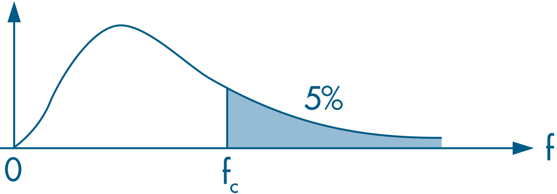
urdenotes the unrestricted model andrdenotes the restricted model.We then evaluate the F statistic using a right-tailed test based on the F distribution:
Implementing It in R
We continue using the
mlb1dataset from Section 4.5 of Wooldridge (2006).The unrestricted model (including all explanatory variables) is \begin{align} \log(\text{salary}) = &\beta_0 + \beta_1. \text{years} + \beta_2. \text{gameyr} + \beta_3. \text{bavg} + \\ &\beta_4 .\text{hrunsyr} + \beta_5. \text{rbisyr} + \varepsilon \end{align}
The restricted model (excluding the variables under test) is \begin{align} \log(\text{salary}) = &\beta_0 + \beta_1. \text{years} + \beta_2. \text{gameyr} + \varepsilon \end{align}
Using linearHypothesis()
- We can compute the F test with
linearHypothesis()from thecarpackage. - Besides the regression object, we must also provide a character vector listing the restrictions:
# Estimating the unrestricted model
res.ur = lm(log(salary) ~ years + gamesyr + bavg + hrunsyr + rbisyr, data=mlb1)

# Creating the vector of restrictions
myH0 = c("bavg = 0", "hrunsyr = 0", "rbisyr = 0")

# Applying the F test
# install.packages("car") # installing the required package
car::linearHypothesis(res.ur, myH0)
## Linear hypothesis test
##
## Hypothesis:
## bavg = 0
## hrunsyr = 0
## rbisyr = 0
##
## Model 1: restricted model
## Model 2: log(salary) ~ years + gamesyr + bavg + hrunsyr + rbisyr
##
##   Res.Df    RSS Df Sum of Sq      F    Pr(>F)
## 1    350 198.31
## 2    347 183.19  3    15.125 9.5503 4.474e-06 ***
## ---
## Signif. codes:  0 '***' 0.001 '**' 0.01 '*' 0.05 '.' 0.1 ' ' 1
- In the second row (the unrestricted model), the residual sum of squares is lower than in the restricted model. So, as expected, the larger set of covariates provides more explanatory power.
- To evaluate the null hypothesis ( $\beta_3 = \beta_4 = \beta_5 = 0$), we can either compare the F statistic with a critical value or check whether the p-value is below the chosen significance level.
- From the p-value criterion above, we reject the null hypothesis.
- The 5% critical value can be obtained with:
qf(1-0.05, G, N-K-1)
## [1] 2.630641
- Since 9.55 > 2.63, we reject the null hypothesis.
Computing It By Hand
- Here we obtain the restricted and unrestricted estimates from
lm()directly, so we do not need to rework every estimation step from scratch.
# Estimating the unrestricted model
res.ur = lm(log(salary) ~ years + gamesyr + bavg + hrunsyr + rbisyr, data=mlb1)

# Estimating the restricted model
res.r = lm(log(salary) ~ years + gamesyr, data=mlb1)

# Extracting the R2 values from the regression results
r2.ur = summary(res.ur)$r.squared
r2.ur
## [1] 0.6278028
r2.r = summary(res.r)$r.squared
r2.r
## [1] 0.5970716
# Computing the F statistic
F = ( r2.ur - r2.r ) / (1 - r2.ur) * (N-K-1) /  G
F
## [1] 9.550254
# F-test p-value
1 - pf(F, G, N-K-1)
## [1] 4.473708e-06