Multivariate OLS Estimation
Estimation with lm()
To estimate a multivariate model in R, we can use the
lm()function:- The tilde (
~) separates the dependent variable from the independent variables. - The independent variables must be separated with
+. - The intercept (
$\beta_0$) is included automatically by
lm(). To remove it, include the “independent variable”0in the formula.
- The tilde (
Example 3.1: Determinants of College GPA in the United States (Wooldridge, 2006)
- Consider the following variables:
colGPA(college GPA): average grade point average in college,hsGPA(high school GPA): average grade point average in high school, andACT(achievement test score): standardized achievement test score used for college admission.
- Using the
gpa1dataset from thewooldridgepackage, we estimate the following model:
$$ \text{colGPA} = \beta_0 + \beta_1 \text{hsGPA} + \beta_2 \text{ACT} + \varepsilon $$
# Loading the gpa1 dataset
data(gpa1, package = "wooldridge")

# Estimating the model and assigning it to an object
GPAres = lm(colGPA ~ hsGPA + ACT, data = gpa1)
GPAres
##
## Call:
## lm(formula = colGPA ~ hsGPA + ACT, data = gpa1)
##
## Coefficients:
## (Intercept)        hsGPA          ACT
##    1.286328     0.453456     0.009426
Coefficients, Fitted Values, and Residuals
We can use the
coef()function to extract a vector with the regression estimates, $\hat{\boldsymbol{\beta}}$.
coef(GPAres)
## (Intercept)       hsGPA         ACT
## 1.286327767 0.453455885 0.009426012
- We can also extract fitted values (
$\hat{\boldsymbol{y}}$) and residuals (
$\hat{\boldsymbol{\varepsilon}} = \boldsymbol{y} - \hat{\boldsymbol{y}}$) using the
fitted()andresid()functions, respectively:
fitted(GPAres)[1:6] # first 6 fitted values
##        1        2        3        4        5        6
## 2.844642 2.963611 3.163845 3.127926 3.318734 3.063728
resid(GPAres)[1:6] # first 6 residuals
##           1           2           3           4           5           6
##  0.15535832  0.43638918 -0.16384523  0.37207430  0.28126580 -0.06372813
- We can extract more detailed information from the regression object (
lm()) using thesummary()function:
summary(GPAres) # detailed regression output
##
## Call:
## lm(formula = colGPA ~ hsGPA + ACT, data = gpa1)
##
## Residuals:
##      Min       1Q   Median       3Q      Max
## -0.85442 -0.24666 -0.02614  0.28127  0.85357
##
## Coefficients:
##             Estimate Std. Error t value Pr(>|t|)
## (Intercept) 1.286328   0.340822   3.774 0.000238 ***
## hsGPA       0.453456   0.095813   4.733 5.42e-06 ***
## ACT         0.009426   0.010777   0.875 0.383297
## ---
## Signif. codes:  0 '***' 0.001 '**' 0.01 '*' 0.05 '.' 0.1 ' ' 1
##
## Residual standard error: 0.3403 on 138 degrees of freedom
## Multiple R-squared:  0.1764,	Adjusted R-squared:  0.1645
## F-statistic: 14.78 on 2 and 138 DF,  p-value: 1.526e-06
summary(GPAres)$coef # estimates, standard errors, t-statistics, and p-values
##                Estimate Std. Error   t value     Pr(>|t|)
## (Intercept) 1.286327767 0.34082212 3.7741910 2.375872e-04
## hsGPA       0.453455885 0.09581292 4.7327219 5.421580e-06
## ACT         0.009426012 0.01077719 0.8746263 3.832969e-01
OLS in Matrix Form
Notation
For more details on the matrix form of OLS, see Appendix E in Wooldridge (2006).
Consider the multivariate model with $K$ regressors for observation $i$: $$ y_i = \beta_0 + \beta_1 x_{i1} + \beta_2 x_{i2} + … + \beta_K x_{iK} + \varepsilon_i, \qquad i=1, 2, …, N \tag{E.1} $$ where $N$ is the number of observations.
Define the parameter column vector, $\boldsymbol{\beta}$, and the row vector of explanatory variables for observation $i$, $\boldsymbol{x}_i$ (lowercase): $$ \underset{1 \times K}{\boldsymbol{x}_i} = \left[ \begin{matrix} 1 & x_{i1} & x_{i2} & \cdots & x_{iK} \end{matrix} \right] \qquad \text{e} \qquad \underset{(K+1) \times 1}{\boldsymbol{\beta}} = \left[ \begin{matrix} \beta_0 \\ \beta_1 \\ \beta_2 \\ \vdots \\ \beta_K \end{matrix} \right],$$
Note that the inner product $\boldsymbol{x}_i \boldsymbol{\beta}$ is:
- Therefore, equation (3.1) can be rewritten, for $i=1, 2, ..., N$, as
$$ y_i = \underbrace{\beta_0 + \beta_1 x_{i1} + \beta_2 x_{i2} + … + \beta_K x_{iK}}_{\boldsymbol{x}_i \boldsymbol{\beta}} + \varepsilon_i = \boldsymbol{x}_i \boldsymbol{\beta} + \varepsilon_i, \tag{E.2} $$
- Let $\boldsymbol{X}$ denote the matrix of all $N$ observations for the $K+1$ explanatory variables:
- We can now stack equations (3.2) for all $i=1, 2, ..., N$ and obtain:
Analytical Estimation in R
Example - Determinants of College GPA in the United States (Wooldridge, 2006)
We want to estimate the model: $$ \text{colGPA} = \beta_0 + \beta_1 \text{hsGPA} + \beta_2 \text{ACT} + \varepsilon $$
Using the
gpa1dataset, we build the dependent-variable vectoryand the independent-variable matrixX:
# Loading the gpa1 dataset
data(gpa1, package = "wooldridge")

# Building the y vector
y = as.matrix(gpa1[,"colGPA"]) # converting the data-frame column into a matrix
head(y)
##      [,1]
## [1,]  3.0
## [2,]  3.4
## [3,]  3.0
## [4,]  3.5
## [5,]  3.6
## [6,]  3.0
# Building the covariate matrix X with a leading column of 1s
X = cbind( const=1, gpa1[, c("hsGPA", "ACT")] ) # combining the constant with the covariates
X = as.matrix(X) # converting to matrix form
head(X)
##   const hsGPA ACT
## 1     1   3.0  21
## 2     1   3.2  24
## 3     1   3.6  26
## 4     1   3.5  27
## 5     1   3.9  28
## 6     1   3.4  25
# Retrieving N and K
N = nrow(gpa1)
N
## [1] 141
K = ncol(X) - 1
K
## [1] 2
1. OLS Estimates $\hat{\boldsymbol{\beta}}$
$$ \hat{\boldsymbol{\beta}} = \left[ \begin{matrix} \hat{\beta}_0 \\ \hat{\beta}_1 \\ \hat{\beta}_2 \\ \vdots \\ \hat{\beta}_K \end{matrix} \right] = (\boldsymbol{X}'\boldsymbol{X})^{-1} \boldsymbol{X}' \boldsymbol{y} \tag{3.2} $$In R:
bhat = solve( t(X) %*% X ) %*% t(X) %*% y
bhat
##              [,1]
## const 1.286327767
## hsGPA 0.453455885
## ACT   0.009426012
2. Fitted Values $\hat{\boldsymbol{y}}$
$$ \hat{\boldsymbol{y}} = \boldsymbol{X} \hat{\boldsymbol{\beta}} \quad \iff \quad \left[ \begin{matrix} \hat{y}_1 \\ \hat{y}_2 \\ \vdots \\ \hat{y}_N \end{matrix} \right] = \left[ \begin{matrix} 1 & x_{11} & x_{12} & \cdots & x_{1K} \\ 1 & x_{21} & x_{22} & \cdots & x_{2K} \\ \vdots & \vdots & \vdots & \ddots & \vdots \\ 1 & x_{N1} & x_{N2} & \cdots & x_{NK} \end{matrix} \right] \left[ \begin{matrix} \hat{\beta}_0 \\ \hat{\beta}_1 \\ \hat{\beta}_2 \\ \vdots \\ \hat{\beta}_K \end{matrix} \right] $$In R:
yhat = X %*% bhat
head(yhat)
##       [,1]
## 1 2.844642
## 2 2.963611
## 3 3.163845
## 4 3.127926
## 5 3.318734
## 6 3.063728
3. Residuals $\hat{\boldsymbol{\varepsilon}}$
$$ \hat{\boldsymbol{\varepsilon}} = \boldsymbol{y} - \hat{\boldsymbol{y}} = \left[ \begin{matrix} y_1 \\ y_2 \\ \vdots \\ y_N \end{matrix} \right] - \left[ \begin{matrix} \hat{y}_1 \\ \hat{y}_2 \\ \vdots \\ \hat{y}_N \end{matrix} \right] \tag{3.3} $$In R:
ehat = y - yhat
head(ehat)
##          [,1]
## 1  0.15535832
## 2  0.43638918
## 3 -0.16384523
## 4  0.37207430
## 5  0.28126580
## 6 -0.06372813
4. Error Variance $s^2$
$$ s^2 = \frac{\hat{\boldsymbol{\varepsilon}}'\hat{\boldsymbol{\varepsilon}}}{N-K-1} \tag{3.4} $$In R, because
$s^2$ is a scalar, it is convenient to convert the “1x1 matrix” into a number with as.numeric():
s2 = as.numeric( t(ehat) %*% ehat / (N-K-1) )
s2
## [1] 0.1158148
5. Variance-Covariance Matrix of the Estimator $\widehat{\text{Var}}(\hat{\boldsymbol{\beta}})$ (or $V_{\hat{\beta}}$)
\begin{align} \widehat{\text{Var}}(\hat{\boldsymbol{\beta}}) &= s^2 (\boldsymbol{X}'\boldsymbol{X})^{-1} \tag{3.5} \\ &= \left[ \begin{matrix} var(\hat{\beta}_0) & cov(\hat{\beta}_0, \hat{\beta}_1) & \cdots & cov(\hat{\beta}_0, \hat{\beta}_K) \\ cov(\hat{\beta}_0, \hat{\beta}_1) & var(\hat{\beta}_1) & \cdots & cov(\hat{\beta}_1, \hat{\beta}_K) \\ \vdots & \vdots & \ddots & \vdots \\ cov(\hat{\beta}_0, \hat{\beta}_K) & cov(\hat{\beta}_1, \hat{\beta}_K) & \cdots & var(\hat{\beta}_K) \end{matrix} \right] \end{align}Vbhat = s2 * solve( t(X) %*% X )
Vbhat
##              const         hsGPA           ACT
## const  0.116159717 -0.0226063687 -0.0015908486
## hsGPA -0.022606369  0.0091801149 -0.0003570767
## ACT   -0.001590849 -0.0003570767  0.0001161478
6. Standard Errors of the Estimator $\text{se}(\hat{\boldsymbol{\beta}})$
They are the square roots of the main diagonal of the estimator’s variance-covariance matrix.
se_bhat = sqrt( diag(Vbhat) )
se_bhat
##      const      hsGPA        ACT
## 0.34082212 0.09581292 0.01077719
Comparing lm() and Analytical Estimation
- Up to this point, we have obtained the estimates $\hat{\boldsymbol{\beta}}$ and their standard errors $\text{se}(\hat{\boldsymbol{\beta}})$:
cbind(bhat, se_bhat)
##                      se_bhat
## const 1.286327767 0.34082212
## hsGPA 0.453455885 0.09581292
## ACT   0.009426012 0.01077719
- We still need to complete the inference step by computing the t-statistics and p-values:
summary(GPAres)$coef
##                Estimate Std. Error   t value     Pr(>|t|)
## (Intercept) 1.286327767 0.34082212 3.7741910 2.375872e-04
## hsGPA       0.453455885 0.09581292 4.7327219 5.421580e-06
## ACT         0.009426012 0.01077719 0.8746263 3.832969e-01
Multivariate OLS Inference
The t Test
After estimation, it is important to conduct hypothesis tests of the form $$ H_0: \ \beta_k = h_k \tag{4.1} $$ where $h_k$ is a constant and $k$ is one of the $K+1$ estimated parameters.
The alternative hypothesis for a two-sided test is $$ H_1: \ \beta_k \neq h_k \tag{4.2} $$ whereas, for a one-sided test, it is $$ H_1: \ \beta_k > h_k \qquad \text{ou} \qquad H_1: \ \beta_k < h_k \tag{4.3} $$
These hypotheses can be conveniently tested with the t test: $$ t = \frac{\hat{\beta}_k - h_k}{\text{se}(\hat{\beta}_k)} \tag{4.4} $$
In practice, we often perform a two-sided test with $h_k=0$ to check whether the estimate $\hat{\beta}_k$ is statistically significant, that is, whether the independent variable has a statistically nonzero effect on the dependent variable:
There are three common ways to evaluate this hypothesis.
(i) The first compares the t statistic with the critical value c for a given significance level $\alpha$: $$ \text{Rejeitamos H}_0 \text{ se:} \qquad | t_{\hat{\beta}_k} | > c. $$
In most applications, we use $\alpha = 5\%$, so the critical value $c$ tends to be close to 2 for a reasonable number of degrees of freedom, approaching the normal critical value of 1.96.
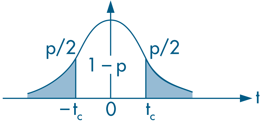
- (ii) Another way to assess the null hypothesis is through the p-value, which indicates how likely it is that $\hat{\beta}_k$ is not an extreme value (that is, how likely it is that the estimate is equal to $a_k = 0$).
$$ p_{\hat{\beta}_k} = 2.F_{t_{(N-K-1)}}(-|t_{\hat{\beta}_k}|), \tag{4.7} $$ where $F_{t_{(N-K-1)}}(\cdot)$ is the CDF of a t distribution with $(N-K-1)$ degrees of freedom.
- Therefore, we reject $H_0$ when the p-value is smaller than the significance level $\alpha$:
- (iii) The third way to assess the null hypothesis is through the confidence interval: $$ \hat{\beta}_k\ \pm\ c . \text{se}(\hat{\beta}_k) \tag{4.8} $$
- In this case, we reject the null when $a_k$ lies outside the confidence interval.
(Continued) Example - Determinants of College GPA in the United States (Wooldridge, 2006)
- Assume $\alpha = 5\%$ and a two-sided test with $a_k = 0$.
7. t Statistic
$$ t_{\hat{\beta}_k} = \frac{\hat{\beta}_k}{\text{se}(\hat{\beta}_k)} \tag{4.6} $$In R:
# Computing the t statistic
t_bhat = bhat / se_bhat
t_bhat
##            [,1]
## const 3.7741910
## hsGPA 4.7327219
## ACT   0.8746263
8. Evaluating the Null Hypotheses
# defining the significance level
alpha = 0.05
c = qt(1 - alpha/2, N-K-1) # critical value for a two-sided test
c
## [1] 1.977304
# (A) Comparing the t statistic with the critical value
abs(t_bhat) > c # evaluating H0
##        [,1]
## const  TRUE
## hsGPA  TRUE
## ACT   FALSE
# (B) Comparing the p-value with the 5% significance level
p_bhat = 2 * pt(-abs(t_bhat), N-K-1)
round(p_bhat, 5) # rounding to improve readability
##          [,1]
## const 0.00024
## hsGPA 0.00001
## ACT   0.38330
p_bhat < 0.05 # evaluating H0
##        [,1]
## const  TRUE
## hsGPA  TRUE
## ACT   FALSE
# (C) Checking whether zero (0) lies outside the confidence interval
ci = cbind(bhat - c*se_bhat, bhat + c*se_bhat) # evaluating H0
ci
##              [,1]       [,2]
## const  0.61241898 1.96023655
## hsGPA  0.26400467 0.64290710
## ACT   -0.01188376 0.03073578
Comparing lm() and Analytical Estimation
- Results computed analytically (“by hand”)
cbind(bhat, se_bhat, t_bhat, p_bhat) # coefficients
##                      se_bhat
## const 1.286327767 0.34082212 3.7741910 2.375872e-04
## hsGPA 0.453455885 0.09581292 4.7327219 5.421580e-06
## ACT   0.009426012 0.01077719 0.8746263 3.832969e-01
ci # confidence intervals
##              [,1]       [,2]
## const  0.61241898 1.96023655
## hsGPA  0.26400467 0.64290710
## ACT   -0.01188376 0.03073578
- Results from the
lm()function
summary(GPAres)$coef
##                Estimate Std. Error   t value     Pr(>|t|)
## (Intercept) 1.286327767 0.34082212 3.7741910 2.375872e-04
## hsGPA       0.453455885 0.09581292 4.7327219 5.421580e-06
## ACT         0.009426012 0.01077719 0.8746263 3.832969e-01
confint(GPAres)
##                   2.5 %     97.5 %
## (Intercept)  0.61241898 1.96023655
## hsGPA        0.26400467 0.64290710
## ACT         -0.01188376 0.03073578
Qualitative Regressors
- Many variables of interest are qualitative rather than quantitative.
- This includes variables such as sex, race, employment status, marital status, brand choice, and so on.
Dummy Variables
- Section 7.1 of Heiss (2020)
- If a qualitative feature is stored as a dummy variable in the dataset (that is, its values are 0s and 1s), it can be included directly in a linear regression.
- When a dummy variable is used in a model, its coefficient represents the difference in intercept between groups (Wooldridge, 2006, Section 7.2).
Example 7.5 - Log Hourly Wage Equation (Wooldridge, 2006)
- We use the
wage1dataset from thewooldridgepackage. - We estimate the model:
\begin{align} \text{wage} = &\beta_0 + \beta_1 \text{female} + \beta_2 \text{educ} + \beta_3 \text{exper} + \beta_4 \text{exper}^2 +\\ &\beta_5 \text{tenure} + \beta_6 \text{tenure}^2 + u \tag{7.6} \end{align} where:
wage: average hourly wagefemale: dummy equal to (1) for women and (0) for meneduc: years of educationexper: years of labor-market experience (expersq= squared experience)tenure: years with the current employer (tenursq= squared tenure)
# Loading the required dataset
data(wage1, package="wooldridge")

# Estimating the model
reg_7.5 = lm(wage ~ female + educ + exper + expersq + tenure + tenursq, data=wage1)
round( summary(reg_7.5)$coef, 4 )
##             Estimate Std. Error t value Pr(>|t|)
## (Intercept)  -2.1097     0.7107 -2.9687   0.0031
## female       -1.7832     0.2572 -6.9327   0.0000
## educ          0.5263     0.0485 10.8412   0.0000
## exper         0.1878     0.0357  5.2557   0.0000
## expersq      -0.0038     0.0008 -4.9267   0.0000
## tenure        0.2117     0.0492  4.3050   0.0000
## tenursq      -0.0029     0.0017 -1.7473   0.0812
- Women (
female = 1) earn, on average, $1.78 less per hour than men (female = 0). - This difference is statistically significant (
femalehas a p-value below 5%).
Variables with Multiple Categories
- Section 7.3 of Heiss (2020)
- When a categorical variable has more than two categories, we cannot simply include it in the regression as though it were a single dummy.
- We need one dummy variable for each category.
- When estimating the model, one category must be omitted to avoid perfect multicollinearity.
- If we know all but one of the dummies, we can infer the value of the remaining dummy.
- If all other dummies are zero, the omitted dummy must equal 1.
- If any other dummy equals 1, then the omitted dummy must equal 0.
- The omitted category becomes the reference group for the estimated coefficients.
Example: Effect of the Minimum-Wage Increase on Employment (Card and Krueger, 1994)
- In 1992, the state of New Jersey (NJ) raised the minimum wage.
- To evaluate whether the increase affected employment, the study used neighboring Pennsylvania (PA) as a comparison group, since it was considered similar to NJ.
- We estimate the following model:
$$ \text{diff_fte} = \beta_0 + \beta_1 \text{nj} + \beta_2 \text{chain} + \beta_3 \text{hrsopen} + \varepsilon $$ where:
diff_fte: change in the total number of employees between February 1992 and November 1992nj: dummy equal to (1) for New Jersey and (0) for Pennsylvaniachain: fast-food chain: (1) Burger King (bk), (2) KFC (kfc), (3) Roy’s (roys), and (4) Wendy’s (wendys)hrsopen: hours open per day
card1994 = read.csv("https://fhnishida.netlify.app/project/rec2312/card1994.csv")
head(card1994) # viewing the first 6 rows
##   sheet nj chain hrsopen diff_fte
## 1    46  0     1    16.5   -16.50
## 2    49  0     2    13.0    -2.25
## 3    56  0     4    12.0   -14.00
## 4    61  0     4    12.0    11.50
## 5   445  0     1    18.0   -41.50
## 6   451  0     1    24.0    13.00
- Notice that the categorical variable
chainuses numeric codes rather than the names of the fast-food chains. - This is common in applied datasets because numbers take less storage space than text.
- If we run the estimation with
chainin this form, the model will treat it as a continuous variable, which leads to an inappropriate interpretation:
lm(diff_fte ~ nj + hrsopen + chain, data=card1994)
##
## Call:
## lm(formula = diff_fte ~ nj + hrsopen + chain, data = card1994)
##
## Coefficients:
## (Intercept)           nj      hrsopen        chain
##     0.40284      4.61869     -0.28458     -0.06462
- The implied interpretation would be that moving from
bk(1) tokfc(2) [or fromkfc(2) toroys(3), or fromroys(3) towendys(4)] reduces the change in employment by a fixed amount, which does not make sense. - Therefore, we need to create dummy variables for the categories:
# Creating one dummy for each category
card1994$bk = ifelse(card1994$chain==1, 1, 0)
card1994$kfc = ifelse(card1994$chain==2, 1, 0)
card1994$roys = ifelse(card1994$chain==3, 1, 0)
card1994$wendys = ifelse(card1994$chain==4, 1, 0)

# Viewing the first few rows
head(card1994)
##   sheet nj chain hrsopen diff_fte bk kfc roys wendys
## 1    46  0     1    16.5   -16.50  1   0    0      0
## 2    49  0     2    13.0    -2.25  0   1    0      0
## 3    56  0     4    12.0   -14.00  0   0    0      1
## 4    61  0     4    12.0    11.50  0   0    0      1
## 5   445  0     1    18.0   -41.50  1   0    0      0
## 6   451  0     1    24.0    13.00  1   0    0      0
- It is also possible to create dummies more conveniently with the
fastDummiespackage. - Notice that with only three chain columns, we can infer the fourth, because each store can belong to only one of the four chains and therefore there is only one
1in each row. - If we include all four dummies in the regression, we create a perfect multicollinearity problem:
lm(diff_fte ~ nj + hrsopen + bk + kfc + roys + wendys, data=card1994)
##
## Call:
## lm(formula = diff_fte ~ nj + hrsopen + bk + kfc + roys + wendys,
##     data = card1994)
##
## Coefficients:
## (Intercept)           nj      hrsopen           bk          kfc         roys
##    2.097621     4.859363    -0.388792    -0.005512    -1.997213    -1.010903
##      wendys
##          NA
- By default, R omits one category to serve as the reference group.
- Here,
wendysis the reference category for the other dummy estimates.- Relative to
wendys, the employment change for:bkis very similar (only 0.005 lower),roysis lower by roughly 1 worker, andkfcis lower by roughly 2 workers.
- Relative to
- We could choose a different fast-food chain as the reference category by omitting a different dummy.
- Let us omit the
roysdummy:
lm(diff_fte ~ nj + hrsopen + bk + kfc + wendys, data=card1994)
##
## Call:
## lm(formula = diff_fte ~ nj + hrsopen + bk + kfc + wendys, data = card1994)
##
## Coefficients:
## (Intercept)           nj      hrsopen           bk          kfc       wendys
##      1.0867       4.8594      -0.3888       1.0054      -0.9863       1.0109
- Now the coefficients are interpreted relative to
roys:- the estimate for
kfc, which had been about -2, is now less negative (about -1), - the estimates for
bkandwendysare now positive (remember that, relative towendys, the estimate forroyswas negative in the previous regression).
- the estimate for
In R, it is not actually necessary to create dummies manually if the categorical variable is stored as text or as a
factor.Creating a character variable:
card1994$chain_txt = as.character(card1994$chain) # creating a character variable
head(card1994$chain_txt) # viewing the first values
## [1] "1" "2" "4" "4" "1" "1"
# Estimating the model
lm(diff_fte ~ nj + hrsopen + chain_txt, data=card1994)
##
## Call:
## lm(formula = diff_fte ~ nj + hrsopen + chain_txt, data = card1994)
##
## Coefficients:
## (Intercept)           nj      hrsopen   chain_txt2   chain_txt3   chain_txt4
##    2.092109     4.859363    -0.388792    -1.991701    -1.005391     0.005512
- Notice that
lm()drops the category that appears first in the character vector ("1"). - With a character variable, it is not easy to choose which category is omitted from the regression.
- To control that choice, we can use a
factorobject:
card1994$chain_fct = factor(card1994$chain) # creating a factor variable
levels(card1994$chain_fct) # checking the factor levels (categories)
## [1] "1" "2" "3" "4"
# Estimating the model
lm(diff_fte ~ nj + hrsopen + chain_fct, data=card1994)
##
## Call:
## lm(formula = diff_fte ~ nj + hrsopen + chain_fct, data = card1994)
##
## Coefficients:
## (Intercept)           nj      hrsopen   chain_fct2   chain_fct3   chain_fct4
##    2.092109     4.859363    -0.388792    -1.991701    -1.005391     0.005512
- Note that
lm()drops the first factor level from the regression (not necessarily the first category appearing in the raw dataset). - We can change the reference group with the
relevel()function on afactorvariable.
card1994$chain_fct = relevel(card1994$chain_fct, ref="3") # using Roy's as the reference
levels(card1994$chain_fct) # checking the factor levels
## [1] "3" "1" "2" "4"
# Estimating the model
lm(diff_fte ~ nj + hrsopen + chain_fct, data=card1994)
##
## Call:
## lm(formula = diff_fte ~ nj + hrsopen + chain_fct, data = card1994)
##
## Coefficients:
## (Intercept)           nj      hrsopen   chain_fct1   chain_fct2   chain_fct4
##      1.0867       4.8594      -0.3888       1.0054      -0.9863       1.0109
- Notice that the first level was changed to
"3", so that category is the one omitted from the regression.
Interactions Involving Dummies
Interactions Between Dummy Variables
- Subsection 6.1.6 of Heiss (2020)
- Section 7 of Wooldridge (2006)
- By adding an interaction term between two dummies, we can obtain different estimates for one dummy (a change in the intercept) across the two categories of the other dummy (0 and 1).
(Continued) Example 7.5 - Log Hourly Wage Equation (Wooldridge, 2006)
Returning to the
wage1dataset from thewooldridgepackage,we now include the dummy variable
married.The model to be estimated is:
\begin{align} \log(\text{wage}) = &\beta_0 + \beta_1 \text{female} + \beta_2 \text{married} + \beta_3 \text{educ} +\\ &\beta_4 \text{exper} + \beta_5 \text{exper}^2 + \beta_6 \text{tenure} + \beta_7 \text{tenure}^2 + u \end{align} where:
wage: average hourly wagefemale: dummy equal to (1) for women and (0) for menmarried: dummy equal to (1) for married individuals and (0) for single individualseduc: years of educationexper: years of labor-market experience (expersq= squared experience)tenure: years with the current employer (tenursq= squared tenure)
# Loading the required dataset
data(wage1, package="wooldridge")

# Estimating the model
reg_7.11 = lm(lwage ~ female + married + educ + exper + expersq + tenure + tenursq, data=wage1)
round( summary(reg_7.11)$coef, 4 )
##             Estimate Std. Error t value Pr(>|t|)
## (Intercept)   0.4178     0.0989  4.2257   0.0000
## female       -0.2902     0.0361 -8.0356   0.0000
## married       0.0529     0.0408  1.2985   0.1947
## educ          0.0792     0.0068 11.6399   0.0000
## exper         0.0270     0.0053  5.0609   0.0000
## expersq      -0.0005     0.0001 -4.8135   0.0000
## tenure        0.0313     0.0068  4.5700   0.0000
## tenursq      -0.0006     0.0002 -2.4475   0.0147
In this regression, marriage has a positive but statistically insignificant effect of 5.29% on wages.
This lack of significance may reflect heterogeneous marriage effects: wages may rise for men while falling for women.
To allow the marriage effect to differ by sex, we can interact
marriedandfemale:lwage ~ female + married + married:female(the:adds only the interaction), orlwage ~ female * married(the*adds the dummies and the interaction).
The model to be estimated now is: \begin{align} \log(\text{wage}) = &\beta_0 + \beta_1 \text{female} + \beta_2 \text{married} + \delta_2 \text{female*married} + \beta_3 \text{educ} + \\ &\beta_4 \text{exper} + \beta_5 \text{exper}^2 + \beta_6 \text{tenure} + \beta_7 \text{tenure}^2 + u \end{align}
# Estimating the model - specification (a)
reg_7.14a = lm(lwage ~ female + married + female:married + educ + exper + expersq + tenure + tenursq,
               data=wage1)
round( summary(reg_7.14a)$coef, 4 )
##                Estimate Std. Error t value Pr(>|t|)
## (Intercept)      0.3214     0.1000  3.2135   0.0014
## female          -0.1104     0.0557 -1.9797   0.0483
## married          0.2127     0.0554  3.8419   0.0001
## educ             0.0789     0.0067 11.7873   0.0000
## exper            0.0268     0.0052  5.1118   0.0000
## expersq         -0.0005     0.0001 -4.8471   0.0000
## tenure           0.0291     0.0068  4.3016   0.0000
## tenursq         -0.0005     0.0002 -2.3056   0.0215
## female:married  -0.3006     0.0718 -4.1885   0.0000
# Estimating the model - specification (b)
reg_7.14b = lm(lwage ~ female * married + educ + exper + expersq + tenure + tenursq,
               data=wage1)
round( summary(reg_7.14b)$coef, 4 )
##                Estimate Std. Error t value Pr(>|t|)
## (Intercept)      0.3214     0.1000  3.2135   0.0014
## female          -0.1104     0.0557 -1.9797   0.0483
## married          0.2127     0.0554  3.8419   0.0001
## educ             0.0789     0.0067 11.7873   0.0000
## exper            0.0268     0.0052  5.1118   0.0000
## expersq         -0.0005     0.0001 -4.8471   0.0000
## tenure           0.0291     0.0068  4.3016   0.0000
## tenursq         -0.0005     0.0002 -2.3056   0.0215
## female:married  -0.3006     0.0718 -4.1885   0.0000
- Notice that the coefficient on
marriednow refers only to men, and it is positive and significant at 21.27%. - For women, the marriage effect is $\beta_2 + \delta_2$, which equals -8.79% (= 0.2127 - 0.3006).
- An important hypothesis is H$_0:\ \delta_2 = 0$, which tests whether the intercept shift associated with marital status differs between women and men.
- In the regression output, the interaction coefficient (
female:married) is significant, so the effect of marriage on women is statistically different from the effect on men.
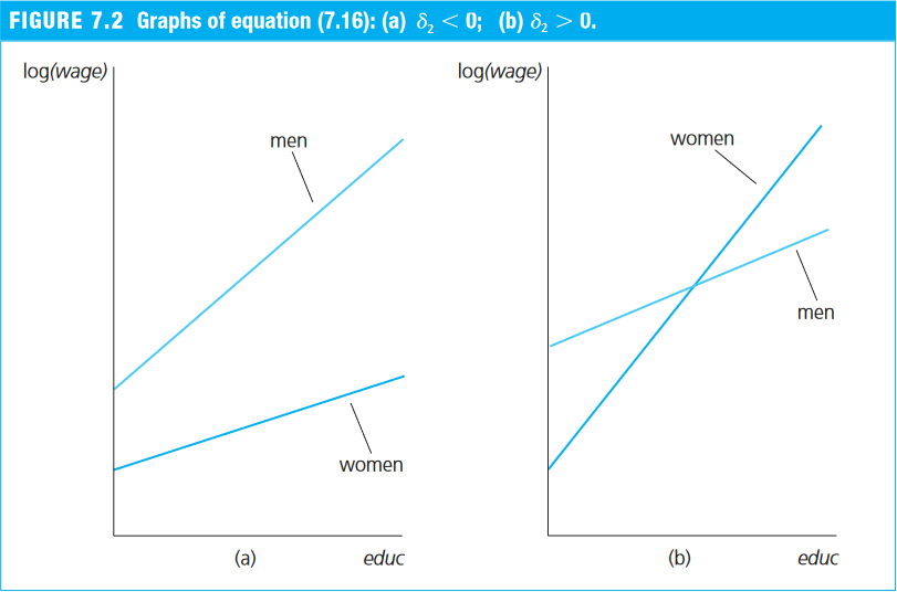
Allowing for Different Slopes
- Section 7.4 of Wooldridge (2006)
- Section 7.5 of Heiss (2020)
- By adding an interaction term between a continuous variable and a dummy, we can allow the coefficient on the continuous variable (that is, the slope) to differ across the two categories of the dummy (0 and 1).
Example 7.10 - Log Hourly Wage Equation (Wooldridge, 2006)
- Returning again to the
wage1dataset from thewooldridgepackage, - we suspect that women not only have a different intercept than men, but also lower wage returns to an additional year of education.
- We therefore include the interaction between the
femaledummy and years of education (educ):
\begin{align} \log(\text{wage}) = &\beta_0 + \beta_1 \text{female} + \beta_2 \text{educ} + \delta_2 \text{female*educ} \\ &\beta_3 \text{exper} + \beta_4 \text{exper}^2 + \beta_5 \text{tenure} + \beta_6 \text{tenure}^2 + u \end{align} where:
wage: average hourly wagefemale: dummy equal to (1) for women and (0) for meneduc: years of educationfemale*educ: interaction between thefemaledummy and years of education (educ)exper: years of labor-market experience (expersq= squared experience)tenure: years with the current employer (tenursq= squared tenure)
# Loading the required dataset
data(wage1, package="wooldridge")

# Estimating the model
reg_7.17 = lm(lwage ~ female + educ + female:educ + exper + expersq + tenure + tenursq,
              data=wage1)
round( summary(reg_7.17)$coef, 4 )
##             Estimate Std. Error t value Pr(>|t|)
## (Intercept)   0.3888     0.1187  3.2759   0.0011
## female       -0.2268     0.1675 -1.3536   0.1764
## educ          0.0824     0.0085  9.7249   0.0000
## exper         0.0293     0.0050  5.8860   0.0000
## expersq      -0.0006     0.0001 -5.3978   0.0000
## tenure        0.0319     0.0069  4.6470   0.0000
## tenursq      -0.0006     0.0002 -2.5089   0.0124
## female:educ  -0.0056     0.0131 -0.4260   0.6703
- An important hypothesis is H$_0:\ \delta_2 = 0$, which tests whether the return to an extra year of education (the slope) differs between women and men.
- The estimates imply that the wage return for women is 0.56 percentage points lower than for men:
- Men receive an 8.24% return (
educ) for each additional year of education. - Women receive a 7.58% return (= 0.0824 - 0.0056) for each additional year of education.
- Men receive an 8.24% return (
- However, this difference is not statistically significant at the 5% level.