Simple OLS Regression
- Section 2.1 of Heiss (2020)
- Consider the following empirical model: $$ y = \beta_0 + \beta_1 x + u \tag{2.1} $$
- According to Wooldridge (2006, Section 2.2), the ordinary least squares (OLS) estimators are given by
- The fitted (predicted) values, $\hat{y}$, are given by $$ \hat{y} = \hat{\beta}_0 + \hat{\beta}_1 x \tag{2.4} $$ such that $$ y = \hat{y} + \hat{u} $$
Example 2.3: CEO Compensation and Stock Returns (Wooldridge, 2006)
- Consider the following simple regression model:
$$ \text{salary} = \beta_0 + \beta_1 \text{roe} + u $$
where
salaryis CEO compensation in thousands of dollars androeis the return on equity, measured in percentage points.
Estimating Simple Regression “By Hand”
# Load the dataset from the 'wooldridge' package
data(ceosal1, package="wooldridge")

attach(ceosal1) # avoids writing 'ceosal1$' before every variable

cov(salary, roe) # covariance between the dependent and independent variables
## [1] 1342.538
var(roe) # variance of the return on equity
## [1] 72.56499
mean(roe) # mean return on equity
## [1] 17.18421
mean(salary) # mean salary
## [1] 1281.12
# Compute the OLS coefficients "by hand"
( b1_hat = cov(salary, roe) / var(roe) ) # by (2.3)
## [1] 18.50119
( b0_hat = mean(salary) - var(roe)*mean(salary) ) # by (2.2)
## [1] -91683.31
detach(ceosal1) # stop looking for variables inside the 'ceosal1' object
- We see that a one-percentage-point increase in return on equity (
roe) is associated with an increase of about 18 thousand dollars in CEO compensation.
Estimating Simple Regression with lm()
- A more convenient way to estimate an OLS model is to use the
lm()function. - In a univariate model, we write the dependent and independent variables separated by a tilde (
~):
lm(ceosal1$salary ~ ceosal1$roe)
##
## Call:
## lm(formula = ceosal1$salary ~ ceosal1$roe)
##
## Coefficients:
## (Intercept)  ceosal1$roe
##       963.2         18.5
- We can also omit the
ceosal1$prefix by supplyingdata = ceosal1.
lm(salary ~ roe, data=ceosal1)
##
## Call:
## lm(formula = salary ~ roe, data = ceosal1)
##
## Coefficients:
## (Intercept)          roe
##       963.2         18.5
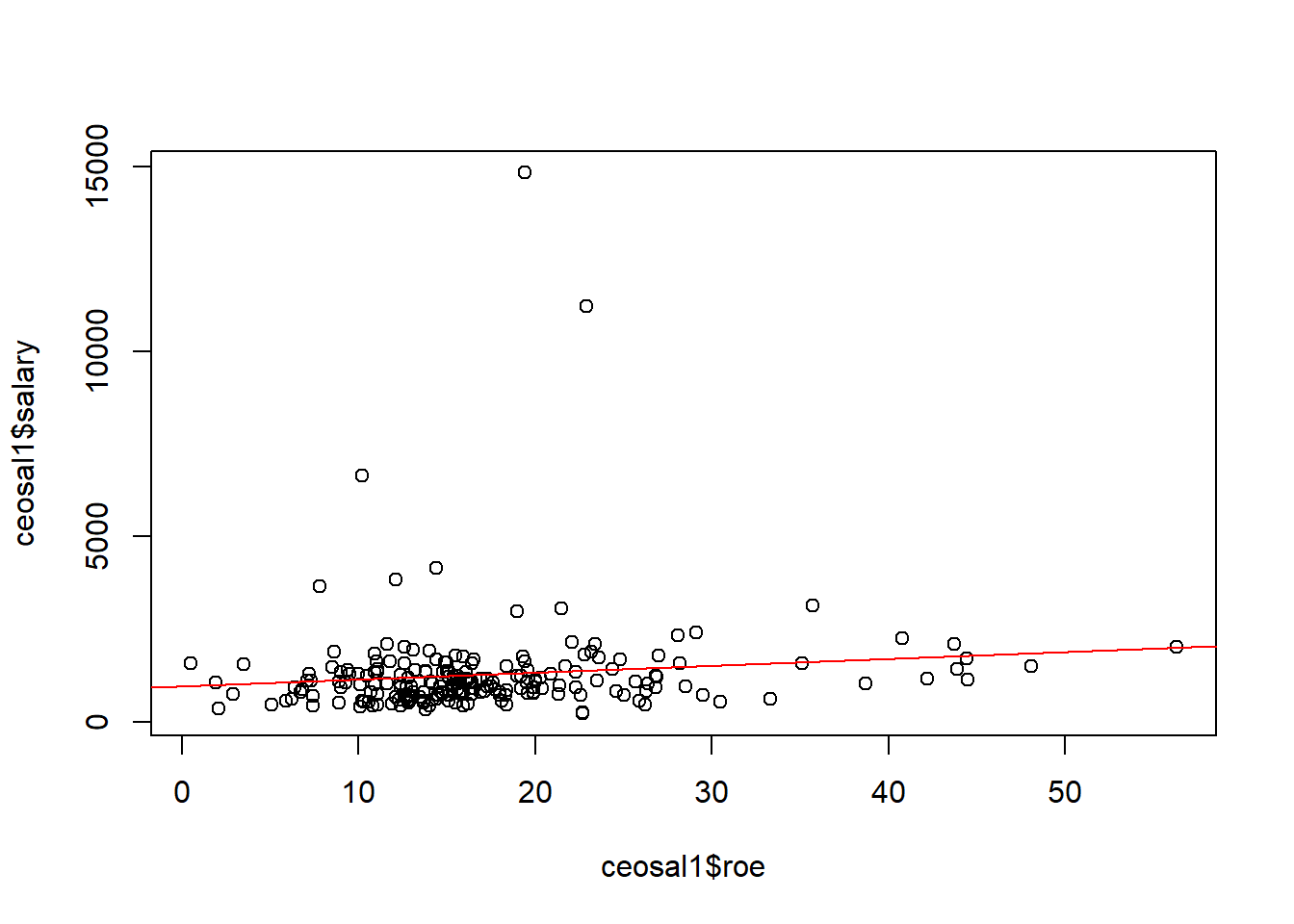
- We can use
lm()to add the regression line to a scatterplot.
# Scatterplot
plot(ceosal1$roe, ceosal1$salary)

# Add the regression line
abline(lm(salary ~ roe, data=ceosal1), col="red")
Coefficients, Fitted Values, and Residuals
- Section 2.2 of Heiss (2020)
- We can store the estimation results in an object (a
list) and then extract information from it.
# Store the regression results in an object
CEOregres = lm(salary ~ roe, data=ceosal1)

# Check the names of the components stored in the object
names(CEOregres)
##  [1] "coefficients"  "residuals"     "effects"       "rank"
##  [5] "fitted.values" "assign"        "qr"            "df.residual"
##  [9] "xlevels"       "call"          "terms"         "model"
- We can use
coef()to extract the estimated regression coefficients.
( bhat = coef(CEOregres) )
## (Intercept)         roe
##   963.19134    18.50119
bhat_0 = bhat["(Intercept)"] # or bhat[1]
bhat_1 = bhat["roe"] # or bhat[2]
- Given these estimated parameters, we can calculate the fitted values, $\hat{y}$, and the residuals, $\hat{u}$, for each observation $i=1, ..., n$:
# Extract ceosal1 columns as vectors
sal = ceosal1$salary
roe = ceosal1$roe

# Compute fitted values
sal_hat = bhat_0 + (bhat_1 * roe)

# Compute residuals
u_hat = sal - sal_hat

# Display the first 6 rows of sal, roe, sal_hat, and u_hat
head( cbind(sal, roe, sal_hat, u_hat) )
##       sal  roe  sal_hat     u_hat
## [1,] 1095 14.1 1224.058 -129.0581
## [2,] 1001 10.9 1164.854 -163.8543
## [3,] 1122 23.5 1397.969 -275.9692
## [4,]  578  5.9 1072.348 -494.3483
## [5,] 1368 13.8 1218.508  149.4923
## [6,] 1145 20.0 1333.215 -188.2151
- With
fitted()andresid(), we can extract the fitted values and residuals directly from the regression object:
head( cbind(fitted(CEOregres), resid(CEOregres)) )
##       [,1]      [,2]
## 1 1224.058 -129.0581
## 2 1164.854 -163.8543
## 3 1397.969 -275.9692
## 4 1072.348 -494.3483
## 5 1218.508  149.4923
## 6 1333.215 -188.2151
# Or equivalently
head( cbind(CEOregres$fitted.values, CEOregres$residuals) )
##       [,1]      [,2]
## 1 1224.058 -129.0581
## 2 1164.854 -163.8543
## 3 1397.969 -275.9692
## 4 1072.348 -494.3483
## 5 1218.508  149.4923
## 6 1333.215 -188.2151
In Section 2.3 of Wooldridge (2006), OLS estimation implies the following sample properties: \begin{align} &\sum^n_{i=1}{\hat{u}_i} = 0 \quad \implies \quad \bar{\hat{u}} = 0 \tag{2.7} \\ &\sum^n_{i=1}{x_i \hat{u}_i} = 0 \quad \implies \quad Cov(x,\hat{u}) = 0 \tag{2.8} \\ &\bar{y}=\hat{\beta}_0 + \hat{\beta}_1.\bar{x} \tag{2.9} \end{align}
We can verify them in our example:
# Checking (2.7)
mean(u_hat) # very close to 0
## [1] -2.666235e-14
# Checking (2.8)
cor(ceosal1$roe, u_hat) # very close to 0
## [1] -6.038735e-17
# Checking (2.9)
mean(ceosal1$salary)
## [1] 1281.12
mean(sal_hat)
## [1] 1281.12
- IMPORTANT: This only means that OLS chooses $\hat{\beta}_0$ and $\hat{\beta}_1$ so that 2.7, 2.8, and 2.9 hold in the sample.
- This does NOT mean that the following population assumptions are necessarily true: \begin{align} &E(u) = 0 \tag{2.7'} \\ &Cov(x, u) = 0 \tag{2.8'} \end{align}
- In fact, if 2.7’ and 2.8’ do not hold, OLS estimation will be biased.
Log Transformations
- Section 2.4 of Heiss (2020)
- We can also estimate models after transforming variables from levels into logarithms.
- This is especially useful for turning nonlinear models into linear ones, such as when the parameter appears in the exponent rather than multiplicatively:
$$ y = A K^\alpha L^\beta\quad \overset{\text{log}}{\rightarrow}\quad \log(y) = \log(A) + \alpha \log(K) + \beta \log(L) $$
- Log transformations are also commonly used for dependent variables with $y \ge 0$.
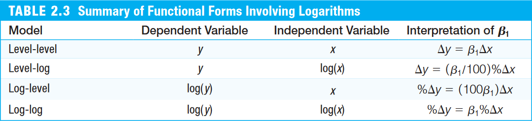
- There are two main ways to apply a log transformation:
- create a new vector/column containing the logged variable, or
- use the
log()function directly insidelm().
Example 2.11: CEO Compensation and Firm Sales (Wooldridge, 2006)
Consider the variables:
wage: annual salary, in thousands of dollarssales: firm sales, in millions of dollars
Level-level model:
# Load the dataset
data(ceosal1, package="wooldridge")

# Estimate the level-level model
lm(salary ~ sales, data=ceosal1)
##
## Call:
## lm(formula = salary ~ sales, data = ceosal1)
##
## Coefficients:
## (Intercept)        sales
##   1.174e+03    1.547e-02
- An increase of US$1 million in sales is associated with an increase of US$0.01547 thousand in CEO compensation.
- Log-level model:
# Estimate the log-level model
lm(log(salary) ~ sales, data=ceosal1)
##
## Call:
## lm(formula = log(salary) ~ sales, data = ceosal1)
##
## Coefficients:
## (Intercept)        sales
##   6.847e+00    1.498e-05
- An increase of US$1 million in sales tends to raise CEO salary by about 0.0015% ($=100 \beta_1%$).
- Log-log model:
# Estimate the log-log model
lm(log(salary) ~ log(sales), data=ceosal1)
##
## Call:
## lm(formula = log(salary) ~ log(sales), data = ceosal1)
##
## Coefficients:
## (Intercept)   log(sales)
##      4.8220       0.2567
- A 1% increase in sales is associated with an increase of about 0.257% in salary ($=\beta_1%$).
Regression Through the Origin and on a Constant
- Section 2.5 of Heiss (2020)
- To estimate the model without an intercept, we need to add
0 +to the regressors insidelm():
data(ceosal1, package="wooldridge")
lm(salary ~ 0 + roe, data=ceosal1)
##
## Call:
## lm(formula = salary ~ 0 + roe, data = ceosal1)
##
## Coefficients:
##   roe
## 63.54
- If we regress a dependent variable on a constant only (
1), we obtain its sample mean.
lm(salary ~ 1, data=ceosal1)
##
## Call:
## lm(formula = salary ~ 1, data = ceosal1)
##
## Coefficients:
## (Intercept)
##        1281
mean(ceosal1$salary, na.rm=TRUE)
## [1] 1281.12
Difference in Means
- Based on Example C.6: the effect of job-training grants on worker productivity (Wooldridge, 2006).
- We can calculate a difference in means by regressing on a dummy variable that takes values 0 or 1.
- First, we create a single vector of scrap rates by stacking
SR87andSR88:
SR87 = c(10, 1, 6, .45, 1.25, 1.3, 1.06, 3, 8.18, 1.67, .98,
         1, .45, 5.03, 8, 9, 18, .28, 7, 3.97)
SR88 = c(3, 1, 5, .5, 1.54, 1.5, .8, 2, .67, 1.17, .51, .5,
         .61, 6.7, 4, 7, 19, .2, 5, 3.83)

( SR = c(SR87, SR88) ) # stack SR87 and SR88 into a single vector
##  [1] 10.00  1.00  6.00  0.45  1.25  1.30  1.06  3.00  8.18  1.67  0.98  1.00
## [13]  0.45  5.03  8.00  9.00 18.00  0.28  7.00  3.97  3.00  1.00  5.00  0.50
## [25]  1.54  1.50  0.80  2.00  0.67  1.17  0.51  0.50  0.61  6.70  4.00  7.00
## [37] 19.00  0.20  5.00  3.83
- Note that the first 20 values refer to scrap rates in 1987 and the last 20 refer to 1988.
- Next, we create a dummy variable called
group88that assigns value 1 to observations from 1988 and 0 to observations from 1987:
( group88 = c(rep(0, 20), rep(1, 20)) ) # 0/1 values for the first/last 20 observations
##  [1] 0 0 0 0 0 0 0 0 0 0 0 0 0 0 0 0 0 0 0 0 1 1 1 1 1 1 1 1 1 1 1 1 1 1 1 1 1 1
## [39] 1 1
- Regressing the scrap rate on the dummy yields the difference in means:
lm(SR ~ group88)
##
## Call:
## lm(formula = SR ~ group88)
##
## Coefficients:
## (Intercept)      group88
##       4.381       -1.154
Expected Values, Variance, and Standard Errors
Wooldridge (2006, Section 2.5) derives the estimator of the error variance: $$ \hat{\sigma}^2 = \frac{1}{n-2} \sum^n_{i=1}{\hat{u}^2_i} = \frac{n-1}{n-2} Var(\hat{u}) \tag{2.14} $$ where $Var(\hat{u}) = \frac{1}{n-1} \sum^n_{i=1}{\hat{u}^2_i}$.
Notice that we need to account for degrees of freedom because we are estimating two parameters ( $\hat{\beta}_0$ and $\hat{\beta}_1$).
Note that $\hat{\sigma} = \sqrt{\hat{\sigma}^2}$ is called the standard error of the regression (SER). In R, this appears as the residual standard error.
We can also obtain the standard errors of the estimators:
Example 2.12: Student Math Performance and the School Lunch Program (Wooldridge, 2006)
Consider the variables:
math10: the percentage of tenth graders who pass a standardized math examlnchprg: the percentage of students eligible for the school lunch program
The simple regression model is $$ \text{math10} = \beta_0 + \beta_1 \text{lnchprg} + u $$
data(meap93, package="wooldridge")

# Estimate the model and store it in the object 'results'
results = lm(math10 ~ lnchprg, data=meap93)

# Extract the number of observations
( n = nobs(results) )
## [1] 408
# Compute the standard error of the regression (square root of 2.14)
( SER = sqrt( (n-1)/(n-2) ) * sd(resid(results)) )
## [1] 9.565938
# Standard error of bhat_0 (2.15)
(1 / sqrt(n-1)) * (SER / sd(meap93$lnchprg)) * sqrt( mean(meap93$lnchprg^2) ) # Standard error of bhat_0
## [1] 0.9975824
(1 / sqrt(n-1)) * (SER / sd(meap93$lnchprg)) # bhat_1
## [1] 0.03483933
- The standard-error calculations can also be obtained with the
summary()function applied to the regression object:
summary(results)
##
## Call:
## lm(formula = math10 ~ lnchprg, data = meap93)
##
## Residuals:
##     Min      1Q  Median      3Q     Max
## -24.386  -5.979  -1.207   4.865  45.845
##
## Coefficients:
##             Estimate Std. Error t value Pr(>|t|)
## (Intercept) 32.14271    0.99758  32.221   <2e-16 ***
## lnchprg     -0.31886    0.03484  -9.152   <2e-16 ***
## ---
## Signif. codes:  0 '***' 0.001 '**' 0.01 '*' 0.05 '.' 0.1 ' ' 1
##
## Residual standard error: 9.566 on 406 degrees of freedom
## Multiple R-squared:  0.171,	Adjusted R-squared:  0.169
## F-statistic: 83.77 on 1 and 406 DF,  p-value: < 2.2e-16
- Also note that, by default,
summary()reports two-sided hypothesis tests whose null hypotheses are $\beta_0 = 0$ and $\beta_1=0$. - In other words, it tests whether the estimated coefficients are statistically equal to zero and reports the corresponding t statistics and p-values.
- In this case, the p-values are extremely small (
<2e-16, that is, smaller than $2 \times 10^{-16}$), so we reject both null hypotheses and conclude that the estimates are statistically significant. - We can also compute these statistics by hand:
# Extract the estimated coefficients
( estim = coef(summary(results)) )
##               Estimate Std. Error   t value      Pr(>|t|)
## (Intercept) 32.1427116 0.99758239 32.220609 6.267302e-114
## lnchprg     -0.3188643 0.03483933 -9.152422  2.746609e-18
# t statistics for H0: bhat = 0
( t_bhat_0 = (estim["(Intercept)", "Estimate"] - 0) / estim["(Intercept)", "Std. Error"] )
## [1] 32.22061
( t_bhat_1 = (estim["lnchprg", "Estimate"] - 0) / estim["lnchprg", "Std. Error"] )
## [1] -9.152422
# p-values for H0: bhat = 0
2 * (1 - pt(abs(t_bhat_0), n-1)) # p-value for bhat_0
## [1] 0
2 * (1 - pt(abs(t_bhat_1), n-1)) # p-value for bhat_1
## [1] 0
Assumption Violations
- Subsection 2.7.3 of Heiss (2020), but using the material from Worked Example 1.
- Simulating a linear model (John Hopkins/Coursera)
- In practice, we run regressions using observed data and do not know the true model that generated those observations.
- In R, however, we can posit a true data-generating process and simulate observations to study what happens when an econometric assumption is violated.
- We will use the example from Worked Example 1, where we want to study the relationship between hours of cooking practice and the number of kitchen burns.
No Assumption Violation: Example 1
- Let $y$ denote the number of kitchen burns and $x$ the number of hours spent learning how to cook.
- Suppose the true model is $$ y = a_0 + b_0 x + \varepsilon, \qquad \varepsilon \sim N(0, 2^2) \tag{1}$$ where $a_0=50$ and $b_0=-5$.
- Set
$a_0$ and
$b_0$, then simulate observations of
$x$ and
$y$.
- For convenience, we generate random draws from $x \sim N(5; 0.5^2)$. Here, the specific distribution of $x$ is not important.
a0 = 50
b0 = -5
N = 200 # number of observations

set.seed(1)
u = rnorm(N, 0, 2) # disturbances: 200 obs. with mean 0 and sd 2
x = rnorm(N, 5, 0.5) # 200 obs. with mean 5 and sd 0.5
y = a0 + b0*x + u # compute y from u and x

plot(x, y)
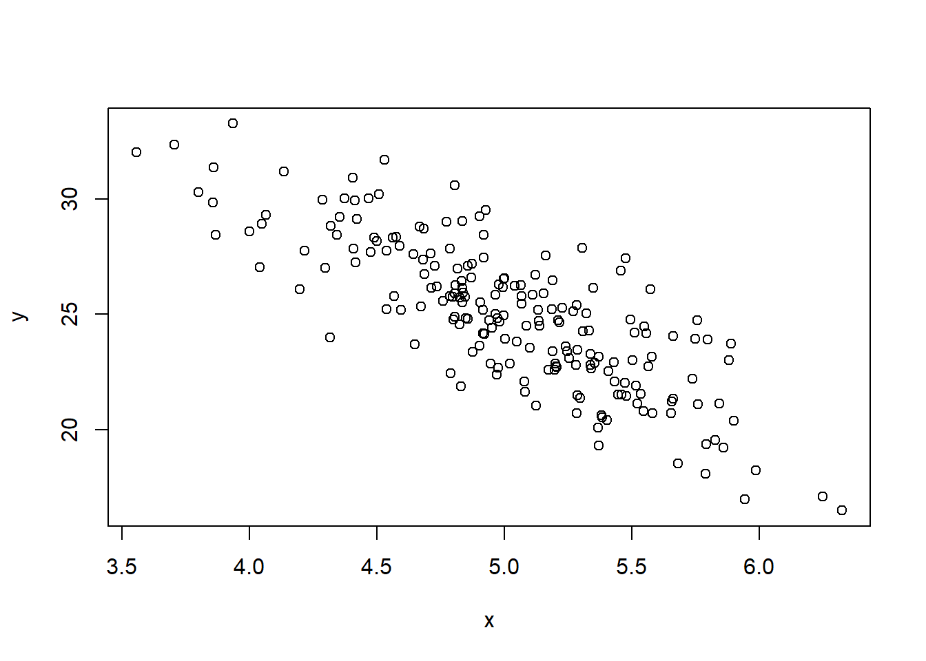 These simulated
$x$ and
$y$ values are the information we would observe in practice.
These simulated
$x$ and
$y$ values are the information we would observe in practice.- Estimate the parameters
$\hat{a}$ and
$\hat{b}$ by OLS using the simulated observations of
$y$ and
$x$.
- Suppose an economist writes the following empirical model: $$ y = a + b x + u, \tag{1a}$$ assuming that $E[u] = 0$ and $E[ux]=0$.
- To estimate the model by OLS, we use
lm().
lm(y ~ x) # regress y on x by OLS
##
## Call:
## lm(formula = y ~ x)
##
## Coefficients:
## (Intercept)            x
##      50.463       -5.078
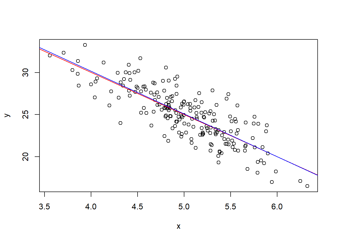
- Notice that the population parameters are recovered reasonably well ( $\hat{a} \approx 50 = a_0$ and $\hat{b} \approx -5 = b_0$).
plot(x, y) # plot x against y
abline(a=50, b=-5, col="red") # true model line
abline(lm(y ~ x), col="blue") # estimated line from the observed data
No Assumption Violation: Example 2
- Now suppose that, in the true model, the number of burns $y$ is determined both by hours of practice $x$ and by hours actually spent cooking $z$:
$$ y = a_0 + b_0 x + c_0 z + u, \qquad u \sim N(0, 2^2) \tag{2} $$ where $a_0=50$, $b_0=-5$, and $c_0=3$. For convenience, we generate random draws from $x \sim N(5; 0.5^2)$ and $z \sim N(1.875; 0.25^2)$. By construction, $z$ is uncorrelated with $x$ in the true model.
- First, let us simulate the observations:
a0 = 50
b0 = -5
c0 = 3
N = 200 # number of observations

set.seed(1)
u = rnorm(N, 0, 2) # disturbances: 200 obs. with mean 0 and sd 2
x = rnorm(N, 5, 0.5) # 200 obs. with mean 5 and sd 0.5
z = rnorm(N, 1.875, 0.25) # 200 obs. with mean 1.875 and sd 0.25
y = a0 + b0*x + c0*z + u # compute y from u, x, and z
Suppose an economist writes the following empirical model: $$ y = a + b x + u, \tag{2a}$$ assuming that $E[u] = 0$ and $E[ux] = 0$.
Notice that the economist omitted the hours-cooking variable $z$, so it is absorbed into the regression error term.
However, because $z$ is unrelated to $x$, this omission does not bias the estimate of $\hat{b}$:
cor(x, z) # correlation between x and z -> close to 0
## [1] -0.02625278
lm(y ~ x) # OLS estimation
##
## Call:
## lm(formula = y ~ x)
##
## Coefficients:
## (Intercept)            x
##       56.27        -5.12
- Since $\hat{b} \approx -5 = b_0$, OLS successfully recovers the population parameter $b_0$ even though the economist excluded $z$ from the model.
- In many economic applications, the main goal is to estimate the relationship or causal effect between $y$ and $x$. We therefore do not need to include every variable that affects $y$, as long as $E(ux) = 0$ holds; that is, as long as no omitted explanatory variable correlated with $x$ is hiding inside the error term.
Violation of E(ux)=0
- Now suppose that, in the true model, the more someone practices cooking, the more time they actually spend cooking. In other words,
$x$ is related to
$z$.
- Assume that $z \sim N(1.875x; (0.25)^2)$:
set.seed(1)
e = rnorm(N, 0, 2) # disturbances: 200 obs. with mean 0 and sd 2
x = rnorm(N, 5, 0.5) # 200 obs. with mean 5 and sd 0.5
z = rnorm(N, 1.875*x, 0.25) # 200 obs. with mean 1.875x and sd 0.25
y = a0 + b0*x + c0*z + e # compute y from e, x, and z
cor(x, z) # correlation between x and z
## [1] 0.9618748
- Now $x$ and $z$ are strongly correlated.
- Estimate the empirical model $$ y = a + b x + u,$$ assuming that $E[u] = 0$ and $E[ux]=0$.
lm(y ~ x) # OLS estimation
##
## Call:
## lm(formula = y ~ x)
##
## Coefficients:
## (Intercept)            x
##     50.6406       0.5053
- Here, $\hat{b} = 0.5 \neq -5 = b_0$. This happens because $z$ was omitted from the model and is therefore absorbed into the residual $\hat{u}$. Since $z$ is correlated with $x$, we have $E(ux)\neq 0$, which violates the key OLS exogeneity assumption.
- If we include $z$ in the regression, we recover an estimate close to $b_0$:
lm(y ~ x + z)
##
## Call:
## lm(formula = y ~ x + z)
##
## Coefficients:
## (Intercept)            x            z
##      50.435       -5.953        3.470
Violation of E(u)=0
- Now assume that $E[u] = k$, where $k \neq 0$ is a constant.
- Let $k = 10$:
a0 = 50
b0 = -5
k = 10

set.seed(1)
u = rnorm(N, k, 2) # disturbances: 200 obs. with mean k and sd 2
x = rnorm(N, 5, 0.5) # 200 obs. with mean 5 and sd 0.5
y = a0 + b0*x + u # compute y from u and x
- If an economist estimates an empirical model that imposes $E[u] = 0$, then:
lm(y ~ x) # OLS estimation
##
## Call:
## lm(formula = y ~ x)
##
## Coefficients:
## (Intercept)            x
##      60.463       -5.078
- Notice that $E[u] \neq 0$ affects the intercept estimate, so $\hat{a} \neq a_0$, but it does not affect $\hat{b} \approx b_0$, which is usually the parameter of primary interest in economic applications.
Violation of Homoskedasticity
- Now suppose that $u \sim N(0, (2x)^2)$, so the variance increases with $x$. In other words, the error variance depends on $x$, and homoskedasticity fails.
a0 = 50
b0 = -5

set.seed(1)
x = rnorm(N, 5, 0.5) # 200 obs. with mean 5 and sd 0.5
u = rnorm(N, 0, 2*x) # disturbances with sd equal to 2x
y = a0 + b0*x + u # compute y from u and x

lm(y ~ x) # OLS estimation
##
## Call:
## lm(formula = y ~ x)
##
## Coefficients:
## (Intercept)            x
##      51.221       -5.166
- Even with heteroskedasticity, we can still recover $\hat{b} \approx b_0$ in this simulation. But with a smaller sample, it becomes more likely that $\hat{b} \neq b_0$. Try repeating the exercise with smaller values of $N$.
Goodness of Fit
- Section 2.3 of Heiss (2020)
- The total sum of squares (TSS), explained sum of squares (ESS), and residual sum of squares (RSS) can be written as
\begin{align} SQT &= \sum^n_{i=1}{(y_i - \bar{y})^2} = (n-1) . Var(y) \tag{2.10}\\ SQE &= \sum^n_{i=1}{(\hat{y}_i - \bar{y})^2} = (n-1) . Var(\hat{y}) \tag{2.11}\\ SQR &= \sum^n_{i=1}{(\hat{u}_i - 0)^2} = (n-1) . Var(\hat{u}) \tag{2.12} \end{align} where $Var(x) = \frac{1}{n-1} \sum^n_{i=1}{(x_i - \bar{x})^2}$.
- Wooldridge (2006) defines the coefficient of determination as \begin{align} R^2 &= \frac{SQE}{SQT} = 1 - \frac{SQR}{SQT}\\ &= \frac{Var(\hat{y})}{Var(y)} = 1 - \frac{Var(\hat{u})}{Var(y)} \tag{2.13} \end{align} because $SQT = SQE + SQR$.
# Compute R^2 in three equivalent ways:
var(sal_hat) / var(sal)
## [1] 0.01318862
1 - var(u_hat)/var(sal)
## [1] 0.01318862
cor(sal, sal_hat)^2 # squared correlation between the dependent variable and fitted values
## [1] 0.01318862
- A more convenient way to obtain
$R^2$ is to use
summary()on the regression object. This produces a more detailed regression table, including $R^2$:
summary(CEOregres)
##
## Call:
## lm(formula = salary ~ roe, data = ceosal1)
##
## Residuals:
##     Min      1Q  Median      3Q     Max
## -1160.2  -526.0  -254.0   138.8 13499.9
##
## Coefficients:
##             Estimate Std. Error t value Pr(>|t|)
## (Intercept)   963.19     213.24   4.517 1.05e-05 ***
## roe            18.50      11.12   1.663   0.0978 .
## ---
## Signif. codes:  0 '***' 0.001 '**' 0.01 '*' 0.05 '.' 0.1 ' ' 1
##
## Residual standard error: 1367 on 207 degrees of freedom
## Multiple R-squared:  0.01319,	Adjusted R-squared:  0.008421
## F-statistic: 2.767 on 1 and 207 DF,  p-value: 0.09777